Key takeaways
ICT explains a retrospective five-minute chart setup around the October 5, 2020 Australian dollar rate statement and cash-rate release at 11:30 p.m.
Read the full summary
ICT explains a retrospective five-minute chart setup around the October 5, 2020 Australian dollar rate statement and cash-rate release at 11:30 p.m. Eastern Time, using the high-impact event to anticipate possible volatility rather than predict its content. Price runs above relative equal highs labeled buy-side liquidity, rejects the breakout, breaks below a selected low to form a bearish breaker, and later retraces during the 8:30 a.m. to 11:00 a.m. New York window. ICT measures an optimal trade entry retracement from the London-session high to a later low and looks for overlap with the bearish breaker, then targets relative equal lows labeled sell-side liquidity and an overlapping projected Fibonacci level. The method combines event timing, a liquidity run, rejection, structural break, measured retracement, session filter, and opposing liquidity target. The example provides no instrument symbol, visible price scale, executable fills, costs, or independently verified results, so it demonstrates a conditional analytical process rather than a validated trading edge.
How we researched this article
BestProps used document-based research from primary firm sources, checked September 25, 2026. The complete source list, scope, limitations, and commercial-state record appear near the end of this article.
In “Blending Price Patterns With Time & Price Theory”, ICT presents a retrospective chart lesson built around an Australian dollar economic release from October 2020. The central idea is not to predict the content of the announcement. Instead, ICT uses the scheduled event to identify when volatility may appear, observes how price behaves around prior highs, and then waits for a later trading window in which two of his patterns overlap.
This is an explanation of ICT’s interpretation of one chart example, not independent evidence that the method has a repeatable trading edge. The captions do not provide the chart’s instrument symbol, visible price scale, executable fills, costs, or independently verified results.
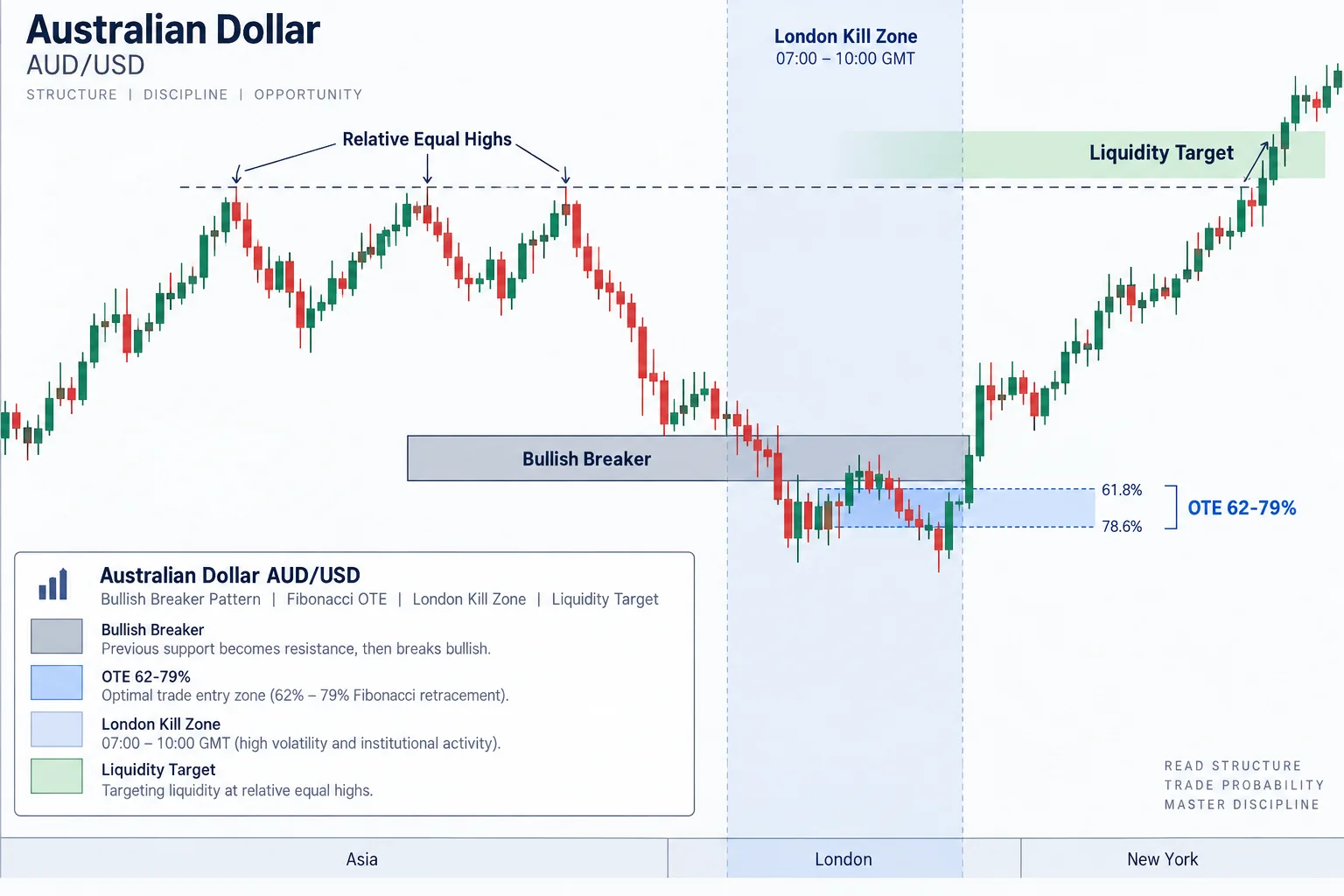
Start with the economic calendar
ICT begins by examining an economic calendar set to Eastern Time. At 0:51, he identifies an RBA rate statement and cash-rate release scheduled for 11:30 p.m. Eastern Time.
He says he is not using the announced, forecast, or previous figures to make a fundamental forecast. Instead, he focuses on the event’s high-impact designation because he expects such events may produce sharp price displacement. In this framework, the calendar supplies a time-based context rather than a directional signal.
That distinction is important: the event does not tell him in advance whether to buy or sell. He waits to see how price behaves around levels already visible on the chart.
The overnight liquidity narrative
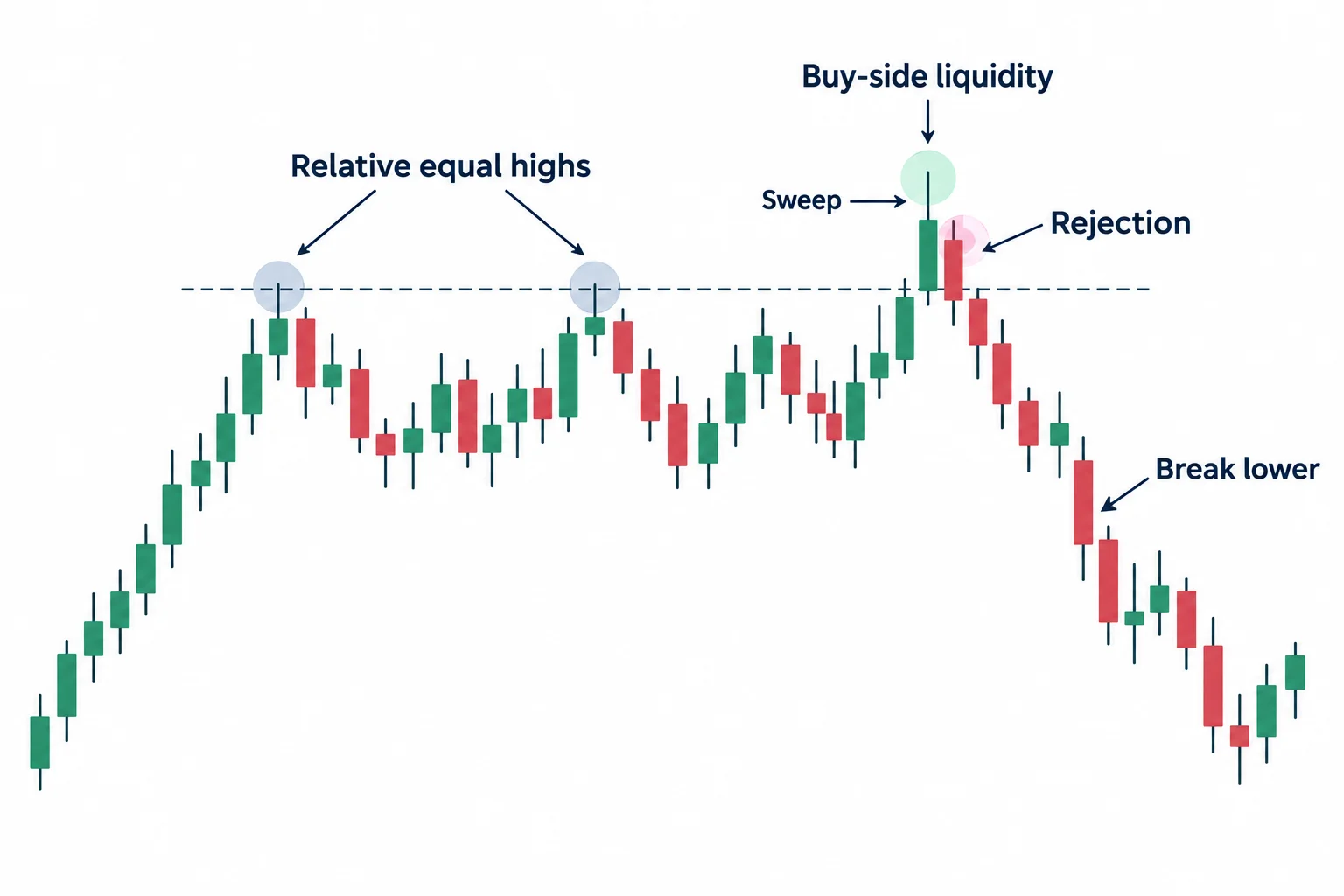
On the five-minute chart, ICT describes a sideways consolidation with several relative equal highs. Beginning around 1:53, he explains that price moved above those highs around the scheduled announcement, rejected the move, and then broke lower.
In ICT terminology, stops and breakout orders above similar highs represent “buy-side liquidity.” His proposed narrative is that the move above the highs could trigger protective stops belonging to short sellers, activate pending breakout-buy orders, fail to remain above the highs, and establish a bearish context once price breaks down.
ICT explicitly says he is not trying to forecast the initial sweep. He first observes whether price trades above the highs and whether it can remain there. The rejection and subsequent decline are what shape his directional interpretation.
How ICT defines the bearish breaker
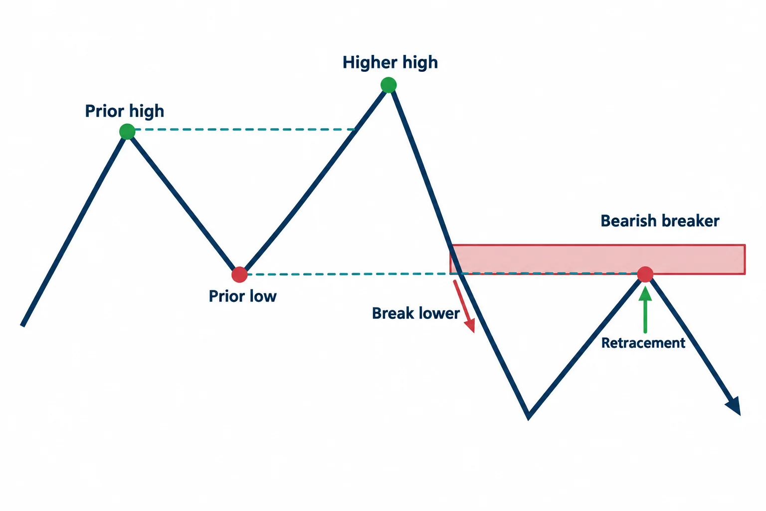
At 2:44, ICT points to a high-low-higher-high sequence and labels it an ICT bearish breaker. He then concentrates on a particular prior low: after that low is broken, he watches for price to retrace to it from below.
He distinguishes this from generic support and resistance. In his explanation, the level matters because of the sequence surrounding it—the run above the equal highs, rejection, bearish break, and return—not merely because price previously turned there. This “narrative” determines which historical low he selects.
Adding time to the price pattern
The second part of the framework is a New York morning window. Around 4:22, ICT specifies 8:30 a.m. to 11:00 a.m. Eastern Time as the period in which he looks for the retracement setup.
He waits for New York trading to revisit the proposed breaker rather than requiring an entry during the earlier London move. This illustrates the lesson’s central idea: a price pattern is not considered in isolation. ICT filters the pattern by asking whether the revisit occurs during his chosen time window.
He also cautions that this 8:30–11:00 window is not identical to what he calls the “New York kill zone.” It is a separate opportunity window used in this example.
Overlap with the optimal trade entry area
ICT next draws a Fibonacci measurement from the London-session high to a later low. At 4:59, he describes the potential short as having two supporting elements:
- a return to the bearish breaker; and
- a return into his Fibonacci-based optimal trade entry area.
He stresses that the Fibonacci tool is a measurement device rather than the cause of the move. The area identified in the captions includes the 79%, 70.5%, and 62% levels. For ICT, the notable feature is the confluence between that retracement zone, the breaker, and the New York time window.
Framing the target
Below the setup, ICT identifies relative equal lows, which he calls “sell-side liquidity.” He also says a projected Fibonacci level aligns with those lows. At 7:10, he presents that overlap as the downside objective after a retracement into the breaker.
The video subsequently shows what ICT describes as a selloff through the equal lows and into the projected target. Because the transcript does not expose chart data or order records, this should be understood as his retrospective chart demonstration—not proof of an executable trade result.
A practical study checklist
For educational chart review, the process presented in the video can be summarized as follows:
- Mark a medium- or high-impact calendar event occurring during the Asian or London period.
- Observe the response instead of predicting direction from the event label.
- Look for a sweep of relative equal highs followed by rejection and a bearish structural break.
- Identify the specific prior low that ICT would classify as a bearish breaker.
- Measure the relevant retracement from the London-session range.
- Wait to see whether the breaker and optimal-entry area overlap between 8:30 and 11:00 a.m. Eastern Time.
- Identify opposing equal lows or another clearly defined objective below.
Near 9:07, ICT summarizes the example as blending two patterns with time-of-day targeting. The transferable lesson is methodological: define the event context, wait for observable price behavior, select levels according to a stated pattern, and then apply a time filter. Traders studying the idea would still need to test its definitions and results independently, including spreads, slippage, failed setups, and alternative interpretations.
Watch the source lesson
ICT’s original video, “Blending Price Patterns With Time & Price Theory,” is available on YouTube.
This link opens the source in a new tab. The video is the property of the Inner Circle Trader channel.
Further reading
- ICT — Blending Price Patterns With Time & Price Theory (source video)
- BabyPips — Forex Market Hours
- Investopedia — Fibonacci Retracement
- BestProps — ICT: High Precision Secrets to Intraday Price Action (Part 2)
Disclaimer: This article is for educational purposes only and is not investment advice. It explains ICT’s interpretation of a chart example; it does not verify trading results or recommend copying any strategy.