Key takeaways
ICT demonstrates a historical Australian dollar setup that blends market structure, a bullish breaker, a 62% to 79% optimal trade entry retracement, the London open kill zone and a buy-side liquidity target.
Read the full summary
ICT demonstrates a historical Australian dollar setup that blends market structure, a bullish breaker, a 62% to 79% optimal trade entry retracement, the London open kill zone and a buy-side liquidity target. At 40 seconds he identifies an October 9 low, high and second low, then shifts from the 15-minute chart to the five-minute chart for clarity. At 1 minute 5 seconds he marks the breaker and OTE overlap, expecting a higher low during the preferred London window. From 2 minutes 38 seconds, a move below equal lows is framed as a sell-side liquidity run, while relative equal highs become the upside objective near 0.72431, with the narrated swing reaching about 0.72432. At 3 minutes 18 seconds, the bullish breaker is defined as the up-close candle before a downswing that makes a lower low, followed by price reclaiming and revisiting that candle. The lesson presents confluence rather than a standalone signal and provides no verified fills, costs, sizing, risk controls, failure rate or evidence of repeatable profitability.
How we researched this article
BestProps used document-based research from primary firm sources, checked September 25, 2026. The complete source list, scope, limitations, and commercial-state record appear near the end of this article.
In Blending Price Patterns With Time & Price Theory [Part 2], ICT walks through a historical Australian dollar chart example that combines a bullish breaker, an optimal trade entry (OTE), a preferred time window and a perceived liquidity objective. The lesson is less about treating any one pattern as a standalone signal and more about showing how ICT layers several concepts into a single market narrative.
ICT Price Patterns Begin With Market Structure
ICT opens by asking viewers to identify a bullish breaker and an OTE in the displayed price action. At 0:40, he describes a low, a high and another low on October 9. He notes that the formation is not especially obvious on the 15-minute chart, so he moves to a five-minute view to make the proposed breaker easier to see.
This change of timeframe is an important part of the demonstration. The broader chart provides context, while the lower timeframe is used to refine the pattern. The transcript does not establish the exact year of the October 9 session, and the video’s October 14, 2020 upload date should not automatically be treated as the chart’s session date.
Blending ICT Price Patterns With Optimal Trade Entry
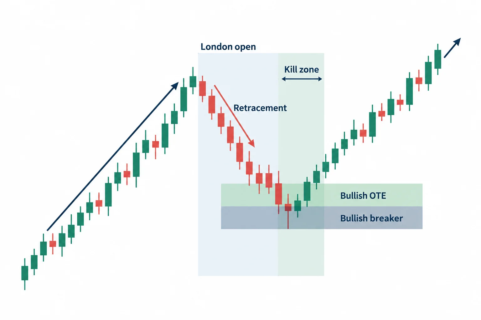
At 1:05, ICT labels the bullish breaker and bullish OTE. He places their overlap within what he calls the London open “kill zone,” a preferred time-of-day window in his framework. His stated expectation is that a bullish market may form a higher low during this period.
ICT then draws a Fibonacci range from the identified low to the high. He describes the OTE area as the retracement between the 62% and 79% levels. The teaching point is the proposed confluence of three elements:
- A bullish directional premise based on the surrounding structure.
- A retracement into ICT’s OTE range.
- An overlap with the London open time window.
These are ICT’s interpretations of the displayed example, not proof that the combination offers a repeatable trading edge. The captions also do not provide entry fills, transaction costs, position sizing or enough information to independently evaluate performance.
ICT Price Objectives Using Liquidity
Beginning around 2:38, ICT zooms out and links the bullish premise to earlier equal lows and relative equal highs. In his terminology, the move beneath the equal lows represents a run on sell-side liquidity. The relative equal highs above price are then treated as buy-side liquidity and as a potential destination for a subsequent advance.
ICT cites a projected high near 0.72431 and says the swing reached approximately 0.72432 before trading lower. Those numbers are statements made in the narration; the transcript alone cannot verify the chart scale, calculation or later price path.
How ICT Price Theory Defines the Bullish Breaker
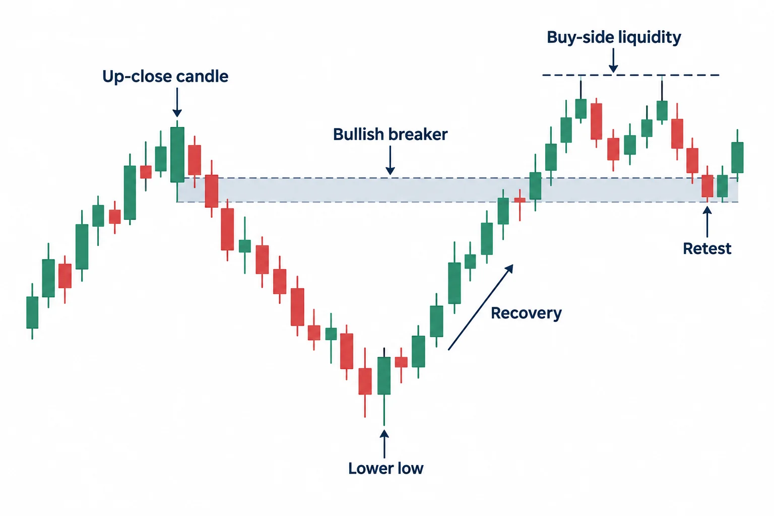
On the five-minute chart, ICT gives a more specific explanation at 3:18. He identifies the up-close candle before a downswing that makes a lower low. In his framework, once price moves back above that candle and later returns to it, the area may act as a bullish breaker.
The breaker is therefore not presented in isolation. ICT pairs it with the low-to-high OTE retracement and the designated time window. He then interprets the advance toward the relative equal highs as an expansion toward buy-side liquidity.
Blending Price Patterns With Time and Objectives
ICT summarizes the example near 4:07 as a low-of-day expansion in bullish conditions, directed toward buy-side liquidity after price had already moved through equal lows. He concludes by emphasizing the combination of two price patterns (the bullish breaker and bullish OTE) with liquidity pools above relative equal highs.
A general educational way to organize the lesson is as a sequence of questions:
- Context: What makes the directional premise bullish or bearish?
- Liquidity event: Has price moved through a prior cluster of similar highs or lows?
- Pattern: Does the lower timeframe show the breaker structure ICT describes?
- Retracement: Does price return to the stated OTE region?
- Timing: Does that retracement overlap the selected session window?
- Objective: Which opposing highs or lows does ICT identify as the draw on liquidity?
This checklist summarizes the logic used in the video; it is not investment advice or a claim that the framework is profitable. The lesson is a compact retrospective chart explanation, and it does not show how often similar-looking setups fail, how signals would be defined without hindsight or what risk controls would be required in live conditions.