How we researched this article
BestProps used document-based research from primary firm sources, checked September 25, 2026. The complete source list, scope, limitations, and commercial-state record appear near the end of this article.
In OTE Pattern Recognition Series – Vol. 15, ICT reviews two Optimal Trade Entry (OTE) examples on a five-minute Australian dollar versus U.S. dollar chart. The chart discussion is used to emphasize a broader lesson: a market can offer opportunities to reduce a position before failing to reach the trader’s final objective.
Watch the full lesson: OTE Pattern Recognition Series – Vol. 15 on YouTube
This summary explains ICT’s interpretation of the setup; it does not establish that OTE has a proven edge. The available source is an automatically transcribed audio track, so the chart’s candles, annotations and displayed prices cannot be independently verified here.
The first AUD/USD OTE example
ICT introduces the lesson as Volume 15 in a planned 20-part pattern-recognition series and asks viewers to inspect the unannotated chart first. He identifies the chart as AUD/USD on the five-minute timeframe and then adds his annotations. See the introduction and chart exercise at 0:10.
At 0:48, he focuses on what he describes as the 8:30 a.m. to 11:00 a.m. New York time window. A downward price leg begins around 8:30, followed by a retracement that ICT classifies as an OTE. Although he also recognizes a smaller retracement as technically qualifying, he gives greater weight to the example aligned with his selected time window.
For the first setup, ICT describes a hypothetical entry at the 62% retracement level, quoted in the audio as 0.6619. He says the position would have experienced approximately four pips of adverse movement and discusses placing a stop ten pips below the referenced low. From there, he evaluates several possible objectives:
- An old high;
- Intermediate areas offering roughly 10 and 20 pips;
- One and one-half standard-deviation projections;
- A two-standard-deviation projection, which he describes as offering about 39 pips.
These figures are ICT’s retrospective reading of the displayed chart, not verified fills or reported trading results. He also notes that the move included a retracement that a trader would have had to withstand.
The secondary entry and the undelivered target
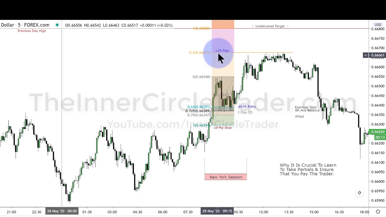
ICT begins a second example at 2:26. Using another low-to-high price leg, he identifies a retracement and gives a hypothetical spread-adjusted entry of 0.6639. He describes approximately three pips of drawdown before price moved above relative equal highs.
According to his narration, the move reached a half-standard-deviation level and offered more than 25 pips. He reads the relevant high as 0.6667 and five “pipettes,” after which the market consolidated and declined. Because the transcription cannot show the price scale, that quotation should be checked against the original chart.
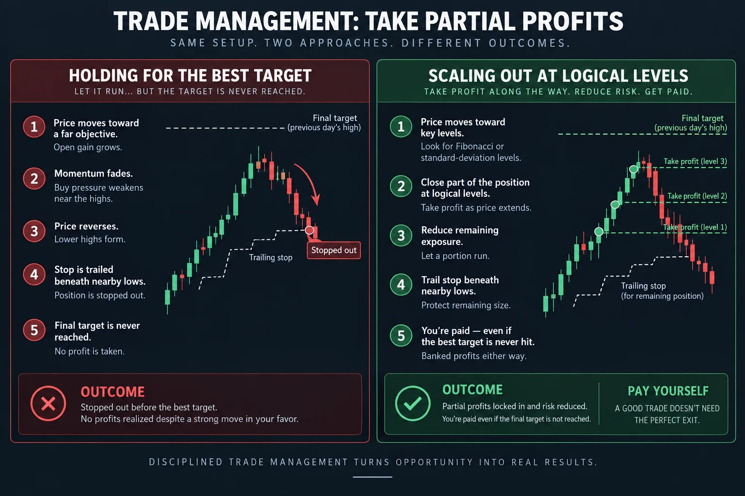
The larger objective was the previous day’s high, quoted as 0.6680. That target was not reached. ICT says a stop trailed beneath nearby lows would eventually have been triggered on any remainder of the position. His central point is that a valid directional idea, in his framework, does not ensure delivery to the most ambitious target.
Why ICT emphasizes partial exits
From 3:41, the lesson shifts from pattern identification to trade management. ICT asks whether reaching a predetermined target matters more than realizing some gain while it is available.
His proposed response is to reduce a position at logical intermediate levels rather than require the entire position to reach a best-case objective. He compares this with receiving pay for part of a workweek: time and effort already expended are not erased simply because the whole week was not completed.
ICT clarifies at 4:58 that the Fibonacci tool is not “magic.” In this presentation, its levels serve as a structured way to identify places where some exposure could be removed. He argues that partial exits can both realize a portion of an open gain and reduce the risk remaining in the market.
General educational interpretation
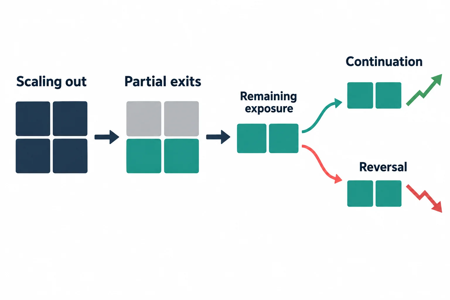
The useful distinction in this lesson is between setup recognition and position management. A trader can define an entry model, stop and distant target, yet still needs rules for what happens between those points. ICT’s example presents scaling out as one possible rule set.
That approach involves a trade-off: taking partial exits reduces exposure to a reversal, but it also reduces participation if price later continues to the final target. The appropriate result cannot be inferred from this single retrospective chart example. Costs, spreads, execution and consistently defined rules would all matter in any broader evaluation.
ICT closes at 7:49 by reiterating that both identified patterns offered, in his assessment, opportunities to take something from the move even though price did not reach the previous day’s high. The episode’s main teaching is therefore not merely how he labels an OTE, but why he does not regard the best-case target as necessary for managing a position.
This article is an educational summary of ICT’s commentary, not investment advice or a promise of trading performance.