How we researched this article
BestProps used document-based research from primary firm sources, checked September 25, 2026. The complete source list, scope, limitations, and commercial-state record appear near the end of this article.
In 2022 ICT Mentorship Episode 23, ICT narrates a Nasdaq 100 futures chart around an FOMC-related period of volatility. The lesson focuses on anticipating an initial decline into a marked area, distinguishing a liquidity sweep from a sustained run through an old high, and reviewing several possible setups after the move.
The recording is best treated as a case study in ICT’s terminology and market interpretation—not as evidence that these concepts provide a proven trading edge. ICT also closes the lesson by warning that FOMC and non-farm payroll periods are extremely risky and are better suited to observation and retrospective study.
The initial FOMC scenario
At 0:06, ICT introduces what he calls the E-mini or Micro Nasdaq 100 market and points to chart imbalances. His proposed sequence is a short-term decline into a lower blue-shaded area, followed by a larger advance through Tuesday’s high.
He explains that he waited several minutes after the FOMC event for the initial “shakeout.” In his interpretation, major scheduled announcements can produce an initial leg, another leg, a false move and then a more useful setup. The chart area he marks is intended to represent where the bearish move may end before price turns higher.
ICT initially discusses a possible short toward a nearby low and sell-side liquidity. At 2:52, he describes a hypothetical stop above the most recent bullish candle to the left. He also identifies a possible bearish order block and a return to a fair value gap as potential reasons for another move lower. These are narrated educational examples; the captions do not establish actual orders or fills.
“Sweep” versus “run”
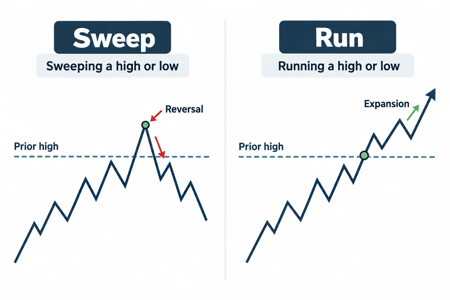
One of the clearest teaching points begins around 4:44. ICT distinguishes between two expressions:
- Sweeping a high or low: Price moves just beyond the level and then reverses back into the prior range.
- Running a high or low: Price trades through the level and continues expanding in the same direction.
ICT characterizes the first shallow move above Tuesday’s high as a sweep. By contrast, his broader expectation is for price to reach the lower target area and then run through Tuesday’s high with stronger continuation. This vocabulary matters because it communicates whether he anticipates rejection at liquidity or expansion beyond it.
The lower target and subsequent review
After pausing the live narration, ICT returns at 7:54 and says price traded into the blue-shaded area, dipped slightly below it and then advanced through Tuesday’s high. This outcome is reported from his chart review in the video; the transcript alone cannot independently verify chart prices, execution or the complete path.
He then explains how he measured the range. He anchors a Fibonacci tool to a high and a later low, identifies the midpoint of that range, and notes that the turquoise fair value gap sits below the 50% level. Once price moves back above the larger fair value gap, he uses the range to project upside objectives.
At 12:02, ICT addresses his choice between candle bodies and wicks. His stated rule for this example is:
- In conditions where he does not expect unusually high volatility, he often measures from the highest opening or closing price to the lowest opening or closing price.
- During an FOMC period, he considers the full extremes—including wicks—because the range is more volatile.
This is ICT’s contextual method rather than a universally established rule. He corrects the drawing direction during the demonstration and redraws from the low to the high because he is looking for upside objectives.
Multiple setups within one price sequence
From 13:27, ICT reconstructs the sequence using his concepts: a liquidity run, a decline into an order block, a rally into a fair value gap, another decline into the previously marked lower area, and then an advance through Tuesday’s high. He also points to later pullbacks into imbalances during the rally.
ICT says he can identify eight possible trades or setups across the broader sequence. The important educational message is not that a viewer should attempt all of them. He explicitly says students are not expected to trade every fluctuation. Instead, he argues that an individual should select one setup whose conditions fit a clearly defined model.
Examples he discusses include a short from a fair value gap, a scalp toward a nearby liquidity objective, a long from the anticipated turning area, a return to an order block, and later continuation entries associated with small imbalances. He excludes the setup immediately before the announcement from his count, calling it a gambler’s setup because it occurs ahead of FOMC volatility.
General educational interpretation
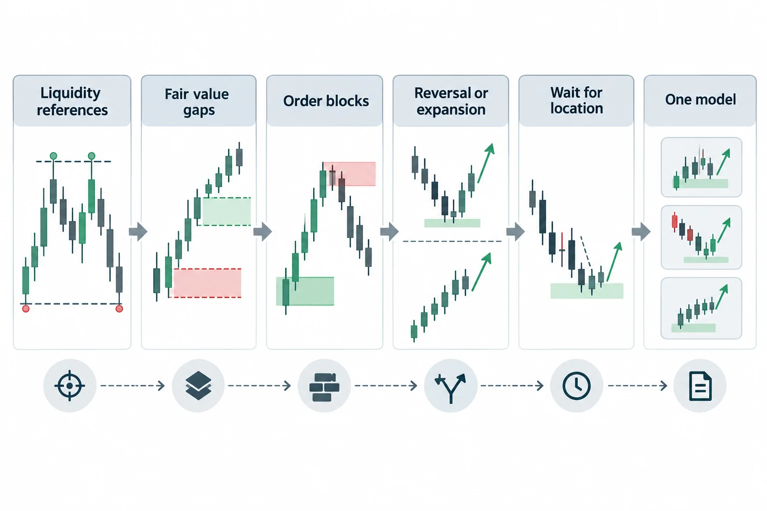
The broader study process presented in the episode can be summarized as follows:
- Mark prior highs and lows that may act as liquidity references.
- Identify imbalances, fair value gaps and order blocks using ICT’s definitions.
- State in advance whether a level is expected to produce a reversal or continued expansion.
- Wait for price to reach the area rather than reacting to every candle.
- Review several possible entries afterward, then narrow them to one repeatable model for further study.
This framework can help organize chart review, but the episode does not provide a controlled test, performance record or basis for assuming profitability. It also does not establish that every FOMC session follows the same sequence.
ICT’s risk warning
At 15:49, ICT emphasizes that the lesson is not an invitation to trade FOMC or non-farm payroll announcements. He describes these events as “very, very risky” and recommends studying how liquidity and range expansion appear either in hindsight or through live observation.
That warning is central to the episode. The video is most appropriately viewed as an explanation of ICT’s chart vocabulary and a reconstruction of one volatile session, not as investment advice or a promise that similar setups will produce the same outcome.
Video
Resources
- ICT Mentorship Episode 23 (YouTube) — Primary source video with full transcript.
- Fair Value Gap Explained (BabyPips) — Independent educational reference for the FVG concept discussed in the episode. Unofficial, not affiliated with ICT.
- Liquidity Definition (Investopedia) — General reference for liquidity terminology used in the lesson. Unofficial, not affiliated with ICT.
- E-mini Nasdaq 100 Futures Specifications (CME Group) — Official contract specifications for the instrument referenced. Unofficial, not affiliated with ICT.