How we researched this article
BestProps used document-based research from primary firm sources, checked September 24, 2026. The complete source list, scope, limitations, and commercial-state record appear near the end of this article.
This is the third lesson in ICT’s commodity trading series, and it surveys the seasonal tendencies he watches across agricultural markets and, later, energy and metals. He states at the start that the material is for paper trading only (0:21) and identifies the recording as the June 2017 ICT Mentorship, commodity trading lesson three, seasonal tendencies: my personal favorites (0:27).
The primary source is ICT Mentorship Core Content – Month 10 – Commodity Seasonals Tendencies – My Personal Favorites, published on YouTube on 17 October 2022 with a running time of about forty-two minutes. The lesson dates its own content to June 2017 and reviews price behaviour up to that year, so every calendar reference below belongs to that period.
The frame he puts around seasonality
His first move is a disclaimer. He says panaceas and be-all end-alls do not exist in trading, and that seasonal tendencies are certainly not one of them (0:44). He is explicit that a trader who places all their faith in seasonality can lose money, and offers his own framing instead: a seasonal tendency is a road map or treasure map that gives a normal expectation of what price action might do at that time of year (1:01). He then gives the obvious reason it can break down — a drought or a bumper crop changes supply, and price goes where supply and demand take it, not where the calendar says (1:34).
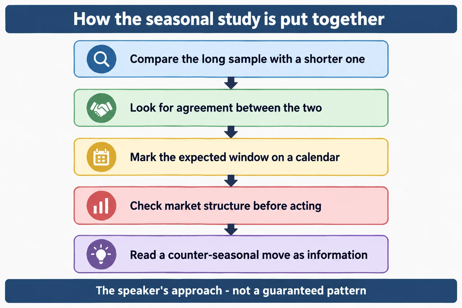
He also describes how the study material is built. Each slide puts a seasonal pattern on the left and a five-year weekly chart on the right, and he deliberately leaves the price charts unmarked so viewers form their own opinion rather than accepting his (2:15). The seasonal charts carry two lines: a solid black line for roughly forty years of seasonal data and a dashed red line for the last fifteen, credited to Steve Moore, whose seasonal resource he is using (5:55). The logic he gives is that if a tendency is real it should show up in both the short sample and the long one, so he looks for the periods where the two lines agree (6:33). He tells viewers not to stop at the five years shown, but to go back as far as the data allows (7:41).
One practical note he adds is about contract selection: trade the first or nearby month because that is where the open interest sits, and check barchart.com to see which contract carries the highest open interest and volume (5:19). He flags gold as an exception that sometimes skips a month late in the year.
Grains and livestock
Soybeans. He describes a rally from around the beginning of February into June or July, a high in that June–July window, then a decline into September or October that forms a seasonal low (3:01). He works through several years on the chart, including a low in January 2013 rallying into July of that year. His most useful point here is what a violation means: if the market is trading lower during its normally bullish first half, that probably reflects an unusually large supply rather than a broken calendar (3:24). He summarises this section at 9:16.
Wheat. He calls this one “a little funky but when it’s there, it’s solid.” The tendency he describes is a decline through the first half of the year and a low forming in late June through August, with a four-to-six-week window in which that low can appear. For bullish conditions he points to lows in the July–August period and again in November as the best times to be a buyer; in a bearish market, the beginning of the year down into the summer months is where he looks for sells (9:56).
Corn. The tendency he draws is a high in May or June and a low in September or October, checked by finding April on the weekly chart and watching for decline into the autumn (13:14). He notes 2016 strength into a September low, and that corn was not declining in spring 2017 — which he reads as underlying relative strength, calling it a possible “sleeper” market rather than dismissing the pattern.
Feeder cattle. A seasonal low in the April–May period that can arrive as early as February, followed by strength into the autumn. He walks through 2013 through 2017, including a 2016 year where he says the seasonal tendency had no impact because of broader bearishness in the market. For context he gives the contract arithmetic: one full point, or 100 basis points, is 500 dollars per contract for feeder cattle (15:33).
Live cattle. A high forming in February–March and a seasonal low in June, with the stronger impulse being a mid-year low followed by a markup into the end of the year (18:05). He shows a July-to-January rally in one year and a June low in another, and notes that in a bearish year the seasonal influence had no effect at all. He says this is a strong one if it can be blended with technical analysis.
Lean hogs. This is one of his stated favourites and the section he is most enthusiastic about. He describes a buy window around March–April that he reads by finding April on the weekly chart and looking one vertical line to the left (March), a high forming in May–July, and a decline into a September–October low (20:39). He calls it the closest thing to perfection in his own study of historical data and one that professional agricultural traders use every year — while also telling viewers to take that with a grain of salt. His enthusiasm is his own reading of past charts; the lesson offers no forward test.
Soft commodities
Cocoa. He admits this pattern is “muddy,” but identifies the best version as a low forming in the last week of May into the first week of June, and a high in the last week of August into September (23:29). He cites a cocoa case study he ran in a live session around the 3,200 to 3,250 level that he says produced doubles and triples on options as a paper trade. That is a reported paper outcome from his own session, not a verified result, and the transcript provides no fills or position details.
Orange juice. A September–October low followed by a rally into December, which he checks by finding October and looking for a low that carries into the January delineation on the left (25:38).
Coffee. He identifies June–July as the best time to be a buyer, with the fifteen-year data favouring mid-June and the forty-year data favouring July (26:23). For bearish conditions he looks for an April–May high, and notes that 2017 had produced exactly that.
Cotton. He describes a strong tendency to sell off in the May period, read off the April section of the weekly chart (28:18). He also gives the counter-reading: in a year where cotton rallied through April–May instead of selling off, that opposing behaviour signalled strong underlying demand, and he notes it kept going higher afterwards.
Energy and metals
Crude oil. An early-year bullish tendency with a seasonal high in the September–October period. He runs through several years and then points at 2017, where there was no seasonal support for upside in the first half and price drifted lower — which he reads, again, as telling you something about supply (30:31).
Copper. He calls this one iffy, like wheat. The buying windows he identifies are June and November, the selling windows September and April (32:15). He notes 2015 had no June–July seasonal low but did sell off in September.
Gold. Simple by his account: a buyer’s market, with the July–August low as the thing to look for, and January–February weakness if someone insists on looking for a short. He attributes the pattern to the physical jewellery cycle — metal has to be mined, processed and made into jewellery in time for the Christmas season (34:26).
Silver. Also a July–August low, with February as a possible selling point, and his preference is to focus on the long side. Here he goes beyond seasonality into a market opinion: he says silver tends to run into a parabolic bull market every ten to twelve years and that he expected it to reach the high twenties over about the following eighteen months (35:51). That is a forecast he made in 2017, stated as his view, and nothing in the recording verifies how it turned out. Treat it as his opinion rather than an established pattern.
His correction about open interest
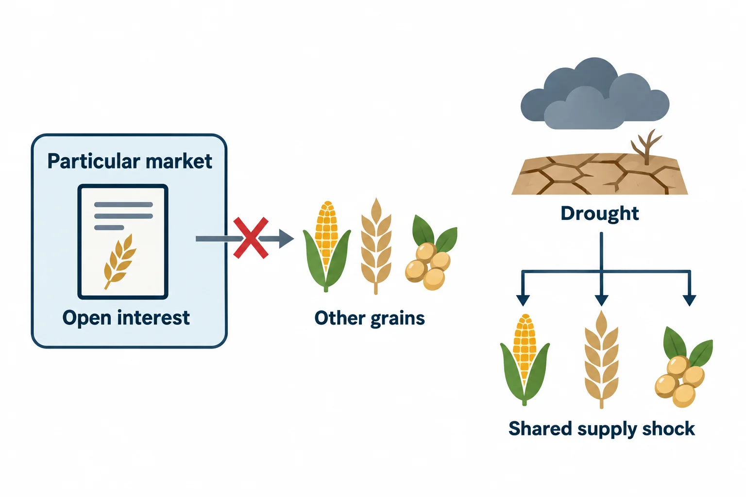
The most instructive part of the lesson is a retraction. He says that in the early 1990s, and in his teaching material at the time, he used declining open interest in thin markets like canola and rice as confirmation that the wider grain complex was bullish. He now says he was very wrong. His explanation is that all the grains were rising simply because a drought pushed all commodities up, and he was erroneously attributing a narrow contract’s open interest decline to wheat, soybeans and corn. He extends the same admission to oats, and states the principle plainly: open interest relates only to that particular market, not to something that can be shared across a complex (38:23).
He also notes the markets he deliberately excludes here — the bond market and debt instruments — because he covers their seasonality separately (38:00).
How he says to use the calendar
His closing process is straightforward: at the start of each month, list the seasonal influences expected for that month, either in a calendar or in your phone. Then open the charts and ask whether there are reasons to justify that seasonal expectation, blending it with the rest of the methodology rather than trading the calendar alone (40:00). He says explicitly not to force it.
The most useful idea he offers is what a failure means. If the seasonal tendency is not working, either the market is in a long-term consolidation — which he says you cannot make money from — or it is moving the opposite way, which tells you something real: significant strength if a bearish window is going up, and strong demand if a bullish window is going down. He suggests checking commercial net-long positioning and the hedging program as cross-checks (41:27).
General educational interpretation
Read as a research method rather than a signal list, the lesson contains a defensible idea and a warning that comes from the speaker himself. The defensible idea is sample agreement: a seasonal pattern that appears in both a long history and a recent sample is a stronger candidate for study than one that only appears in a chosen window. The warning is the open-interest retraction, which is a working example of a plausible-sounding confirmation being discarded once the underlying mechanism is understood. What the lesson does not contain is any statistical test, entry rule, risk limit or verified result, and several of its conclusions rest on the speaker reading charts that viewers cannot see. Anyone studying seasonality would want to reconstruct the series themselves, test the windows out of sample, and treat every stated preference in this lesson as a hypothesis. Futures and options are leveraged; losses can exceed the amount committed. This article is educational commentary, not investment advice.
Watch the original lesson
This article is built from the timestamped English captions of the recording. Captions are a record of the speaker’s words, not independent evidence for anything he reports about markets.
Watch the original lesson on YouTube
The video cannot be played inside another website. When its embedded player was loaded and clicked in a real browser on this page’s behalf on 15 September 2026, the player reported “Playback on other websites has been disabled by the video owner” and offered a “Watch on YouTube” prompt, with no duration and no playback progress. That is why no embed is left blank or half-working here; the recording plays normally on YouTube itself.
Primary source and further reading
- The original Inner Circle Trader lesson: use the timestamp links in this article to compare each explanation with its source.
- CME Group agricultural commodities: the exchange’s product hub for the grain and livestock contracts discussed here, useful for checking which contract months exist and where liquidity sits.
- USDA World Agricultural Supply and Demand Estimates (WASDE): the official monthly supply-and-demand report — the kind of fundamental release that can override a seasonal pattern, which is the risk the lesson itself describes.
- USDA Agricultural Marketing Service market news: continuing public price and volume reporting for agricultural markets, a citable way to reconstruct how a seasonal window actually behaved.
- U.S. Commodity Futures Trading Commission — learning resources: regulator material on futures markets and on evaluating trading claims, including the open-interest concept the lesson discusses.
This is independent educational commentary. It is not official ICT material, a tested seasonal system, or a claim that any described pattern produces results.