
Key takeaways
This is lesson four of the ICT short-term trading module, and it blends two components: what he calls IPDA data ranges, which supply time, and PD arrays, which supply price (0:27).
Read the full summary
This is lesson four of the ICT short-term trading module, and it blends two components: what he calls IPDA data ranges, which supply time, and PD arrays, which supply price (0:27). His lookback windows are 20, 40 and 60 trading days, treated as roughly one, two and three trading months (4:53), rolling forward by one day as each new day is added (0:57). To use them, he splits the relevant high-low range in half and inventories the arrays that actually exist above market price as premium and below it as discount (7:09), working the premium side in the listed order from a likely bearish mitigation block, breaker, liquidity void, fair value gap and bearish order block up to a rejection block and an old high or low (1:39), with the discount side inverted (2:05). Two rules carry most of the weight: arrays he says price has already traded into and reacted to are exhausted, so another reference has to be found (4:31), and the list should never be forced onto a chart — an absent array does not validate or invalidate a setup, it only leaves fewer targets to choose from (5:56). He then walks the Australian dollar daily chart through the three windows (6:23), refines the same week on the four-hour and hourly charts (10:37), and describes switching from an initially bullish Aussie view to a short after Tuesday’s failure swing (11:31), with entries read around a level the captions transcribe as 76.80 and a stated downside objective of 7605 (14:13). It is a live chart lesson, so no entry, fill or result can be reconstructed from the transcript, and nothing here is trading advice.
How we researched this article
BestProps used document-based research from primary firm sources, checked September 24, 2026. The complete source list, scope, limitations, and commercial-state record appear near the end of this article.
Time and price, and why he blends them
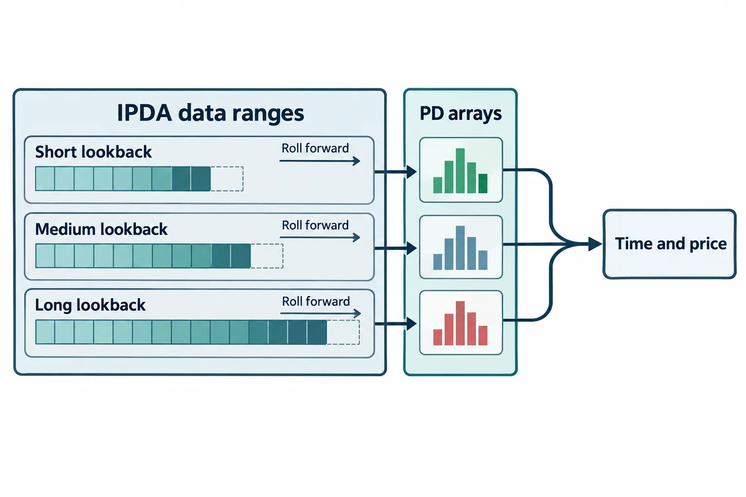
In ICT Mentorship Core Content – Month 07 – Short Term Trading Blending IPDA Data Ranges & PD Arrays, he opens by placing the material: lesson four of the short-term trading module, on blending what he calls IPDA data ranges with PD arrays for liquidity runs (0:09), and he immediately separates the two — the data ranges refer specifically to time, the PD arrays deal specifically with price, so blending them is blending time and price (0:27).
The time component is a rolling lookback of the last 20, the last 40 and the last 60 days (0:51), and he stresses that as each new day arrives you cast forward for a new set of 20, 40 and 60, shifting the range forward by a day (0:57). The purpose he gives is a frame: the lookback gives context in which to place the PD arrays, giving them a reference point in time (1:08). He then names the mechanism in his model — what the captions transcribe as “the enter Bank price delivery algorithm” will reach back into the data arrays across those three windows (1:18), and which window it refers to is respective to the PD array and its position relative to price (1:28). That is his model of how price is delivered, stated as a premise rather than demonstrated; the recording offers no evidence of an algorithm or of who operates it.
The premium and discount arrays, in his stated order
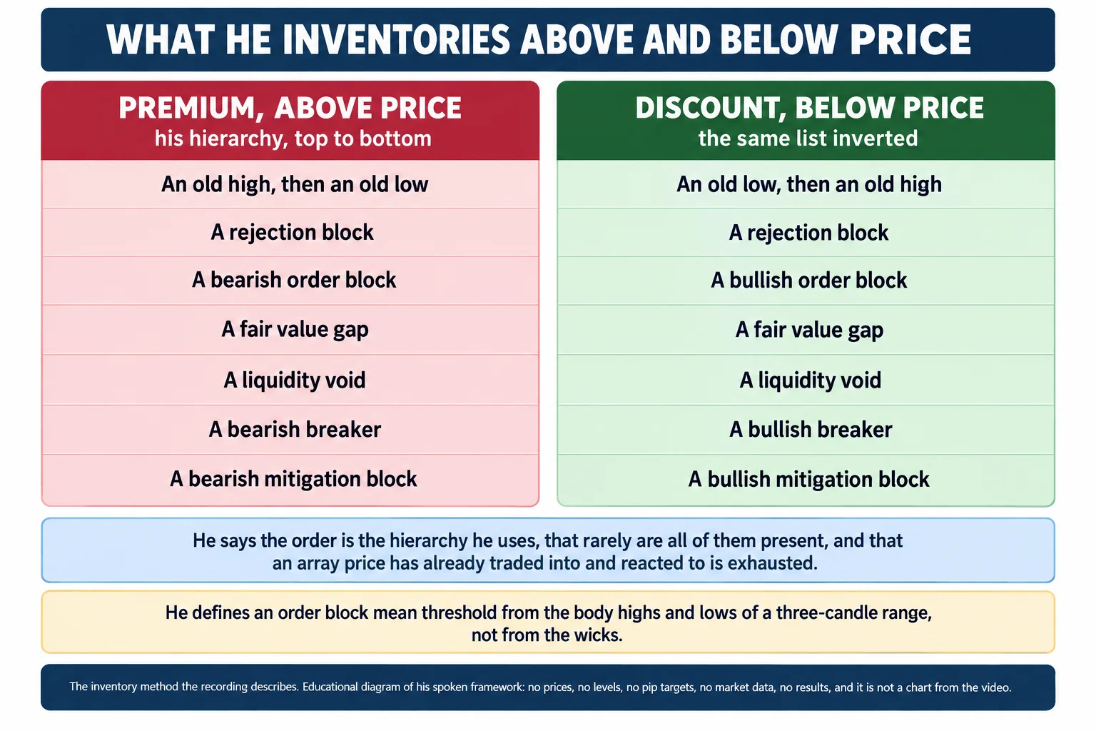
The price component is a list of what he calls PD arrays, split by where price sits in the range. When price is in a premium market, working higher, he says he is looking for a bearish mitigation block, a bearish breaker, a liquidity void, a fair value gap, a bearish order block, a rejection block, and an old high or an old low (1:39). For a discount market he gives the same list inverted: a bullish mitigation block, a bullish breaker, a liquidity void, a fair value gap, a bullish order block, a rejection block, and an old low or old high (2:05).
The order is presented as a sequence rather than a menu. He says the order listed is the order in which the algorithm will seek those references, and that it is not a different order — it is the hierarchy the way they are set up (2:25). He adds the obvious practical caveat: there is not always a void, gap or mitigation block present, and price may simply need to travel all the way up to a bearish order block or a rejection block (2:45), with the same said in opposite terms for a discount market (3:04). He also says the whole thing is not ambiguous once price is viewed through the PD array matrix (3:04).
He is careful about presence and absence. He says rarely do all of the arrays exist, and that a chart may offer a selection of three or four, or as few as two (3:34). The study practice he describes is to start at market price, look at the last 20 days, and ask which premium arrays exist above and which discount arrays exist below (4:06), then repeat over 40 and 60 days (3:11). His line on forcing the idea is direct: the arrays are either in the chart or they are not, and the absence of any one of them does not negate, increase or lessen the validity of an ideal setup — it only means far less to choose from in terms of targets or setups (5:56).
The inventory is time-limited in his framework. If price has already traded down into a bullish order block, responded and reacted accordingly and produced higher prices, he says that PD array has now been exhausted and a different discount array has to be found (4:21). That is the reason the windows have to be re-read as they roll rather than marked once.
Why the windows are treated as one, two and three months
He explains the numbers as approximations against a trading month: 20 trading days as essentially one month, 40 trading days as essentially two months, and 60 trading days as essentially three trading months (4:53). Blending them is what he says gets a trader closest to what the algorithm will seek in terms of trading to the next level of liquidity (5:07).
The directional rule attached is simple. When the market is bearish he works from a premium market down to a discount (5:20), with the premium arrays acting as resistance points, locations of sell signals or sell-offs, or new sell setups (5:34), and the discount arrays as the objectives price is expected to reach (5:34). The inverse would apply for a bullish premise.
The Australian dollar example: building the three windows
The worked example is the Australian dollar on the daily chart (6:23), and the first step he demonstrates is breaking the market up in reference to time (6:39). He marks the lookback windows of 20, 40 and 60 trading days (6:39) and identifies the total 60-day trading range as running from the lowest low noted in that window up to the highest high formed within the last 20 trading days (6:52). Splitting that range in half by its old high and old low is what produces the premium and discount portions of the market (7:09).
He then shows how the windows hand off to one another when price breaks a reference. If the old low is violated, he would go back and look at the old low formed in the 60-day lookback period (7:23); pointing at the arrow delineating the lowest low of the last 20 trading days, he says that if it is violated and traded below, the next lower low or discount array is not in the 40-day window, because there is no lower low there, but in the 60-day lookback (7:32). He also notes that the 40-day range in this example is itself defined by the highest high and the lowest low of the last 20 trading days (8:01).
With the windows drawn, he overlays what he calls the PD array matrix on the 20-day view (8:16) and adds a caveat about the exercise itself: a trader does not need this much information on the chart, and the overlay is a graphic depiction of how he internalises and interprets price action rather than a template to copy (8:30). He defines market price in the example as the Friday close of the week of the recording (8:42) and takes the highest high and lowest low of the last 20 trading days as the first lookback period (9:04).
Working through that 20-day view he lists what he has marked, from the top down: an old high, a rejection block, a bearish order block mean threshold, then the bearish order block, and then down in the discount area a bullish order block, a bullish order block mean threshold, a rejection block, and finally the old low (9:52). The definition he gives for the mean threshold is worth quoting precisely, because it sits inside the terminology rather than being obvious: it is taken from the highs and lows of the bodies of the three candles in the range, not from the wicks, and that is the mean threshold or midway point (10:03).
Stepping down: the four-hour and hourly views
Moving down to a four-hour chart, he says these arrays give much more detail and let a trader start to see how price moves from one array to the next (10:37). The context he then supplies is a failed bullish expectation: the Australian dollar made a higher high on Tuesday, failed to make a higher high and trade higher into a monthly range as he had expected in his analysis (10:51).
What he draws from that failure is the lesson he says matters more than the example. He says a trader does not need to know exactly where the market is going all the time, and that if the analysis fails it gives an immediate reason to consider reversing the analysis and taking trades in the opposite direction (11:06). He applies it to his own week: he had been long or bullish on the Australian dollar, the expectation of a larger price move failed on Tuesday, and once Tuesday broke down the later slides in his presentation offered more analysis suggesting price would trade down and close the liquidity void (11:31).
The mechanical version he states on the four-hour chart is that if price failed on Tuesday and broke down during Tuesday, he starts looking for bearish ideas inside the premium range and keys off the premium PD arrays as potential sell scenarios (11:52), and that when shorting from daily premium arrays he looks to a lesser timeframe — a four-hour or one-hour chart — to target the exit (12:19).
The levels in the example, and their limits
The four-hour view he shows contains a clear liquidity void (12:33), and he points out price trading back up into a mitigation block and a breaker and up to what the captions transcribe as an institutional price level of 76.80 (12:46). His reasoning about not needing the actual high of the week is that a trader can still take part in the move because the shift in order flow has already moved to bearish (12:50), after which the search is for discount PD arrays below (13:10). He describes the void closing and taking price into the discount range (13:18).
A caution belongs here. The caption track does not carry decimal places for these price levels, so 76.80 and 7605 appear exactly as transcribed and this article does not convert them into an assumed decimal form, and it does not treat either figure as a verified level. The precision claim in the recording is likewise left where he puts it: refining the same move into the days of the week on a four-hour chart, he says it came down and closed in the liquidity void right to the pip (13:47). That is the speaker’s own characterisation of his chart, and the transcript cannot substantiate it.
The market maker manipulation template
He then frames the week with a template. Adding what he calls the market maker manipulation template, he describes the high of the week forming on Tuesday at an old monthly, weekly and daily high liquidity pool (13:53), which is what he says happened: price traded slightly above Monday’s high and rejected it, and once Tuesday broke down the likelihood of lower prices was in effect (14:08), which is why he says he called for shorts around the transcribed 76.80 level with a stated downside objective of 7605 (14:13).
The template rule he states is a timeframe relationship: the discount market PD array is used on a timeframe lesser than the premium liquidity pool that was used (14:21). Concretely, the Monday daily high was violated on Tuesday, which he calls a liquidity pool raid on a daily high (14:41), and with that context the next step is to drop to a four-hour or one-hour chart to find the discount array (14:49), which in this case came in the form of the liquidity void taking price down toward the 7605 objective (14:57). He summarises the whole construction as a combination of the time component, the price component and the manipulation templates, used in accordance with the market profiles taught in lesson two, producing a symmetry in the marketplace that would otherwise escape everyone else (15:15).
What the lesson does not establish
This is a live chart lesson recorded during the week he is describing, and he says so, noting the analysis was used in live work that week (15:40). That means the transcript records his commentary over a chart rather than verifiable data: there are no entries, fills, stop levels, transaction costs or account results, and the price levels survive only as the caption track renders them. Nothing here can reconstruct the trades, and the 7605 objective is never followed by a reported outcome in the recording.
He is candid about being wrong. He says the presentation came out of a week in which he was initially wrong about a higher breakout on the Australian dollar, and that the failure swing on Tuesday gave him the insight to change gears and get short on the pair even while it traded in sympathy with a weaker dollar, which he notes is not typical (15:51). The claim that blending time and price lets a trader work within the same parameters as the algorithm at the interbank level is his premise about how markets operate (16:03); the recording supplies no evidence of that mechanism, and the same paragraph of the lesson has already conceded that the trader does not know where the market will go — only that a failed premise can be reversed.
A note on the caption track
This article was written from the video’s own auto-generated caption track, which is the primary source for every timestamp link above. That track mis-recognises several of the speaker’s terms, and they were resolved only where context makes the intended word clear: IPDA appears as “Gupta data ranges” in the opening line and as “the ifta data ranges” at the close (0:15, 16:22), interbank appears as “the enter Bank price delivery algorithm” and elsewhere as “the interbank level” (1:18), and the algorithm he refers to appears simply as “the algorithm” in the passage about trading to the next level of liquidity (5:07). The decimal figures 76.80 and 7605 are reported as transcribed, without converting them. Labels used in this article are the ones the surrounding context supports; nothing was reconstructed from an unintelligible passage, and no array, level or outcome from the recording’s charts is asserted as verified.
Watch the original recording
ICT Mentorship Core Content – Month 07 – Short Term Trading Blending IPDA Data Ranges & PD Arrays
The Inner Circle Trader · published to YouTube on 28 September 2022 · listed as 989 seconds, about 16 minutes 29 seconds. The recording identifies itself as lesson four of the short-term trading module. This video is the primary source for every timestamp link above.
The recording is not embedded here because the video owner has disabled playback on other websites. That was tested directly on 15 September 2026 from a BestProps page origin at both desktop and mobile widths: the embedded player loads and then reports “Playback on other websites has been disabled by the video owner”, with no playable stream in either case. The link above opens the recording on YouTube itself.
Resources
These are the sources checked for this article. The central-bank, market-data and regulator pages are general reference material; none of them assesses the speaker, verifies the IPDA lookback windows, the PD array hierarchy or the transcribed price levels above, or endorses anything said in the recording. The internal calculator link was already present on this page and is retained as a general BestProps tool. Any ICT, smart-money or third-party indicator, script, note set, transcript pack, chart annotation or re-upload circulating outside the publishing channel’s own page is unofficial and untested here.
- [1] ICT Mentorship Core Content – Month 07 – Short Term Trading Blending IPDA Data Ranges & PD Arrays — The Inner Circle Trader (primary source; watch page read 15 September 2026, listed at 989 seconds).
- [2] The Inner Circle Trader — official YouTube channel (read 15 September 2026) — the publishing channel for the ICT mentorship series, including the short-term trading module this lesson belongs to.
- [3] Reserve Bank of Australia — Exchange Rates (read 15 September 2026) — the RBA’s own published rate data for the Australian dollar, the currency pair used in the lesson’s example and the pair whose levels the caption track does not carry decimals for.
- [4] BestProps — Trading Day Requirement Calculator (read 15 September 2026) — an educational calculator for counting trading days, relevant background to the lesson’s use of 20, 40 and 60 trading-day windows rather than calendar days. General tool, not evidence about the method.
- [5] CF