
Key takeaways
This recording is lesson eight of ICT’s short-term-trading module and it is the One Shot One Kill model for the final week of March 2017.
Read the full summary
This recording is lesson eight of ICT’s short-term-trading module and it is the One Shot One Kill model for the final week of March 2017. He presents it as a procedure, not a pattern: work out the current or possible next quarterly shift, read the higher-time-frame arrays inside the 20, 40 and 60 trading-day ranges, check whether the interest-rate markets are trending or stuck in consolidation, scan seasonal tendencies through the calendar year, classify swings from the higher time frames down to the 60-minute chart, decide which weekly profile is likely — for a bearish week naming a Monday high, a Tuesday high or a Wednesday reversal — then map premium and discount around the midpoint of a chosen range, sell into a premium array and aim at an opposing discount array, confirming with intermarket analysis. His euro-dollar example rests on a March seasonal tendency for weakness into early April, commercial positioning he plots himself from the weekly Commitment of Traders report, a dollar index he read as bullish from a weekly discount array, and euro-pound sold off all week. He says he called the weekly high at 109.08 and a 106.50 low objective, and he says the high should land on Monday, Tuesday or Wednesday. The numbers are his own narration of what he posted that week. The captions show no fills, no account results and no independently verified outcome, and he states plainly at the end that there is no clear-cut application that works the same way every time.
How we researched this article
BestProps used document-based research from primary firm sources, checked September 24, 2026. The complete source list, scope, limitations, and commercial-state record appear near the end of this article.
What the lesson actually sets out to be
The recording opens by identifying itself as lesson eight of the short-term-trading module and as the last of March’s content, then asks what One Shot One Kill requires to be done “efficiently and successfully” (0:10, 0:12, 0:20). The answer he gives is a prerequisite list rather than an entry rule: familiarity with the macro conditions and the January lessons, the ability to read data ranges looking back over the last 20, 40 and 60 trading days, price-delivery array concepts applied to both time and price, position and swing trading concepts, the short-term tutorials on his website, Power of Three applied to weekly candles or ranges, the intraday concepts from his day-trading modules, the day-of-week idea, Fibonacci targeting, session timing or kill zones, seasonal change, and Commitment of Traders analysis with commercial hedging programmes (0:37, 0:46, 1:19, 1:35, 1:52, 2:09).
Two things he says about the lesson are worth separating from the technique itself. The first is that it is deliberately a fill-in-the-gaps module rather than a standalone system, and he tells the viewer the prerequisite is to have worked through the free tutorials first (2:16, 2:27, 2:41). The second is the problem the procedure is meant to solve: he describes students who accumulate a great deal of information and then flounder, asking themselves whether they have too much information, and he attributes that to not having had a procedural way of using it (5:47, 5:51). He calls the procedure itself a “back of a matchbook” idea — short, and made of things the viewer should already know (5:07, 5:14).
The procedure in the order he gives it
From about 6:20 he walks the sequence with euro-dollar as the working example. It begins with determining the current or potentially next quarterly shift, then identifying the higher-time-frame price-delivery arrays inside the data ranges — both of which he flags as January content (6:26, 6:34).
Next comes the interest-rate read, and his rule of thumb is mechanical: if rates, Treasuries or the Bund are trending, movement is permitted in euro-dollar, and if they are consolidated and tight, it becomes very hard for the market to move around (6:44, 6:55, 7:05). That is his stated interpretation, not an established relationship, and he does not present data for it in this recording.
He then scours the calendar year for seasonal windows that offer high odds of a move either way, and classifies the price swings from the higher time frames down to the 60-minute chart, on the reasoning that larger trends break into smaller swings, an impulse followed by an expansion after a retracement. The output of that step is a decision about which swings to use for projections, measurements and retracements (7:13, 7:24, 7:41, 7:52).
The weekly profile follows. If he is looking for lower prices he wants a template that allows a bearish idea, and he names the first candidates as the Monday high of the week, the Tuesday high of the week, and a Wednesday reversal. Only then does he move to the market-maker manipulation templates for the matching profile characteristics, determine where premium and discount sit in the price action, and wait for volatility to signal that range expansion is likely — his stated preference being to get in while the market is quiet so the expansion has room to run (7:59, 8:17, 8:27, 8:41, 8:48).
Positioning and confirmation close the sequence. Commitment of Traders data in the commercials versus the large traders, plus open interest, is used to confirm what he calls smart-money action; the trade is framed as a low-resistance liquidity run with opposing arrays, selling short at a premium array for a bearish idea and pairing it with a discount array as the objective; Fibonacci levels converging with those arrays supply the location; and intermarket analysis confirms the setup (9:14, 9:21, 9:26, 9:31, 9:44, 10:05).
The seasonal half of the argument
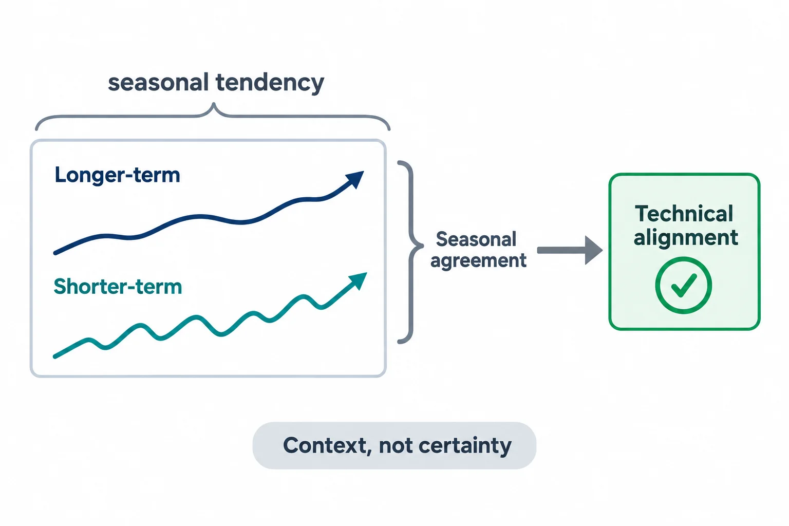
His seasonal case is built on the euro-dollar chart for March, which he describes as rallying into the middle of the month and then declining through the last week of March into the first week of April. He reads that as a strong seasonal tendency for bearish euro prices, and his condition for trusting a tendency is that the longer-term and shorter-term trend lines — which he calls the blue and the red lines — agree on direction (13:49, 14:02, 14:06, 13:40).
He then states the limit of that tool in the plainest terms in the recording: a seasonal tendency is not the be-all and end-all, it illustrates a probable condition or probable outcome, and there has to be something lining up technically to put it in sync with the market. Without that, he says, the seasonal tendency will get you in trouble (22:24, 22:22, 22:26, 22:40). It is the same qualification that appears in his other teaching, and it is the sentence that keeps the rest of this lesson in proportion.
The commitment-of-traders construction he describes
The part of the lesson he is most emphatic about is not publicly available in the form he uses, and he says so: it is not on the internet, it is not in books, and he builds it himself. His description is that he takes the Commitment of Traders report data, looks back over the last calendar year, takes the highest high and the lowest low of the commercials’ net positions only, and uses those to construct what he calls a new zero-sum line. He says he tracks 39 markets but that it takes him seconds on the two pairs he focuses on, and that he creates the line by hand from the report rather than running an indicator (14:15, 14:19, 14:39, 14:56, 15:01, 15:08).
He also states which participants he ignores and why. Commercial traders are the banks, large institutions and producers, and the CFTC requires traders above a reportable level to disclose their buying, selling and net positions; he says he does not look at the large traders or the small speculators (16:03, 16:09, 16:14, 16:21, 16:28). Later in the lesson, his summary is that you need two things coupled for what he calls smart money, and that open interest is not that important here because two factors are already blended (20:55, 21:01, 21:11).
The euro-dollar example, and what it does and does not establish
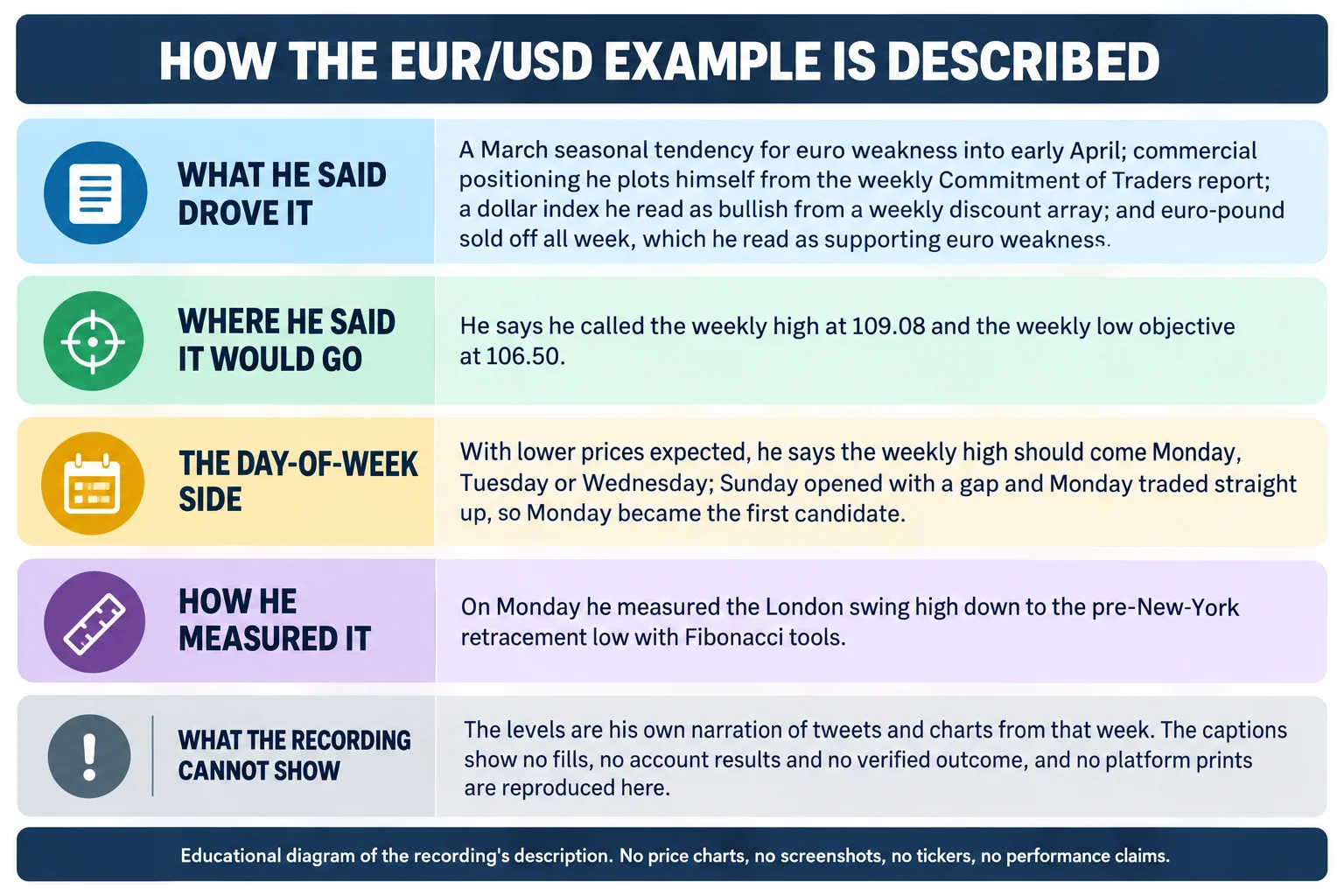
The case study is introduced as a setup provided to the viewers in the last week of March 2017, and he says he outlined through tweets and videos that he expected a high to form around 109.08. He then reports the outcome he observed: the actual high was 109.09 on the platform he names, he projected a 106.50 low for the week with a 106.95 intermediate objective, and he says Friday’s close pushed the pair down to 106.55, with some traders in his live feeds getting 106.497, and he leaves it to the viewer to determine what their own data provider printed (10:15, 10:26, 10:35, 10:45, 10:50, 11:06, 11:22, 11:38, 11:42). Those figures are reported by the speaker about that week. They are not independently verified here, and no fills or account results are established anywhere in the captions.
The confluence he lists for the bearish idea is the seasonal window, the commercial positioning in his own chart, a dollar index he read as trading up off a weekly discount array after trading down into an old weekly high, and euro-pound sold aggressively all week into a four-hour bullish order block, which he treats as euro weakness and pound strength (22:43, 23:12, 23:21, 26:15, 26:23, 26:46, 27:09). On the dollar index he also describes a checklist of draws — liquidity pools, bearish order blocks, fair value gaps, mitigation blocks, breakers, old highs and old lows acting as resistance — and says all were traded to except the fair value gap, which he expected to be reached on the following Sunday or Monday (24:14, 24:33, 24:44).
The day-of-week side, and the leeway he insists on
With the bearish case assembled, he says the expectation becomes a weekly high on Monday, Tuesday or Wednesday, and that you always start with Monday because it is the first day of the week (28:53, 29:01, 29:07). Sunday opened with a gap and price traded straight up on Monday into the weekly bearish order block, so he assumed Monday was the weekly high (27:23, 27:31, 27:51, 29:12, 29:18).
He is careful, though, to say he does not try to time the weekly high precisely, and to explain why: it can go up on Tuesday and make a higher high, so the idea needs leeway. His suggestion is to sell a very small portion on Monday, so that if Tuesday fails to make a higher high there is a small piece on at the higher level, and if it does go higher on Tuesday or Wednesday the position is not fully underwater (29:25, 29:30, 29:39, 29:50, 30:01).
The measurement he describes for that Monday is intraday: price traded up and then retraced, with a London retracement and an expansion through New York, and he measured the swing from the London high down to the retracement low before the New York rally with Fibonacci tools, which gave him 109.09. He says he then used one pip below it and called it 109.08 precisely because he is usually about a pip off, and notes the market went to the actual level on the platform he names (30:11, 30:29, 30:44, 30:48, 31:03). He frames the Monday rally as a false rally engineered higher so that what he calls smart money could sell into it (31:34, 31:41). That is his interpretation of the move, offered as an explanation rather than demonstrated.
The range construction he shows on the four-hour chart is explicit: take the 106.50 level as the baseline, draw up to the projected weekly high of 109.08, divide the range in half for an equilibrium price point, and treat everything above it as premium and everything below as discount. The objective he names is a liquidity void at the lower end of the discount range (31:56, 32:10, 32:15, 32:20, 25:06, 32:35).
His own closing qualifications
The end of the lesson is the part most worth keeping. He says plainly that there is not going to be a clear-cut way to do this every single time, that there will be decisions to make, and he gives a concrete version of the problem: you might think the weekly high is in on Monday, sell short, and then watch Tuesday in London or New York run up and blow that high out. His question to the viewer is whether you stick with the idea or get whipsawed into reversing (33:31, 33:50, 33:53).
What he recommends instead is study in hindsight, looking back over 10, 15 or 20 years of data to build a mental library of past outcomes, and he says a daily chart is enough for that rather than every detail down to the hourly (34:29, 34:35, 34:48, 34:59). He also describes the model as something to reduce down through position, swing, short-term and day-trading horizons, and he closes by saying the lesson is intended to fill in the gaps in his free short-term tutorials (36:53, 37:02, 37:25).
A checklist drawn from the lesson
This is a general educational ordering of what he describes, not a tested system and not his own wording:
- Establish the quarterly context and read the higher-time-frame arrays inside the 20, 40 and 60 trading-day ranges.
- Note whether the rate markets are trending or consolidating, and treat that as context rather than a signal.
- Find the seasonal window that applies and require technical alignment before using it.
- Choose the weekly profile you expect and name which day the weekly extreme is most likely to form on.
- Map premium and discount around the midpoint of a defined range, then locate a premium array to sell into and a discount array as the objective.
- Size so that being early is survivable, which is the leeway he describes for the day-of-week assumption.
Anyone comparing this framework across dates should note that the day-of-week figure he gives — the track renders it as “76 odds” of the high or low forming Monday through Wednesday — is stated as a given, with no sample, method or source offered in the recording (1:39). It belongs in the same category as the seasonal read: a working assumption the speaker uses, not a result established here.
A note on the captions
The transcript used for this article is the automatic YouTube caption track for the recording, not a human-checked transcript, and it mishears several terms. Where the track is plainly wrong and context makes the intended word unambiguous, the term has been normalised: “the ifta data ranges” and “the if the data ranges” are the data ranges, “seasonal tenancy” and “season Tendencies” are seasonal tendency and seasonal tendencies, “CRT” where he goes on to say Commitment of Traders is the Commitment of Traders report, “premium PDA” and “discount PDA” are premium and discount price-delivery arrays, “downed candles” is down-close candles, and “the police has been insightful” is the lesson has been insightful. Where the track is ambiguous the wording has been described rather than quoted. The level numbers in the euro-dollar example are reproduced as the track gives them because he states them more than once, but they remain his reported figures, not verified market data. The recording also contains long stretches where he is describing charts on screen, and this article reports only what he says about them.
Watch the original recording
ICT Mentorship Core Content – Month 07 – One Shot One Kill Model
The Inner Circle Trader · published 1 October 2022 · about 38 minutes. This recording is the primary source for every timestamp link above.
The recording is not embedded here because the video owner has disabled playback on other websites. That was tested directly on 15 September 2026 from a BestProps page origin at both desktop and mobile widths: the embedded player loads, then reports “Playback on other websites has been disabled by the video owner” with no duration and no playback progress, while the video itself plays normally on YouTube. No empty or half-working player is left on this page.
The watch page was read on 15 September 2026 and is publicly listed as ICT Mentorship Core Content – Month 07 – One Shot One Kill Model by The Inner Circle Trader, upload date 1 October 2022, listed duration 2,259 seconds — about 37 minutes, 39 seconds. The caption track used for this article runs to 2,258.54 seconds, so the transcript and the listed duration agree. The upload date is separate from the period the lesson discusses: the recording presents itself as the last of March’s content for that mentorship year, and its euro-dollar example is set in the final week of March 2017.
Resources
These are the sources checked for this article. The regulator and exchange pages are general material about how futures and forex markets are regulated and how trading systems sold to the public should be assessed; none of them evaluates this speaker, verifies any array, level, seasonal read or positioning chart described above, or endorses anything said in the recording. Any ICT, smart-money or third-party indicator, script, note set, chart annotation, transcript pack or re-upload circulating outside the publishing channel’s own page is unofficial and has not been tested here.
- [1] ICT Mentorship Core Content – Month 07 – One Shot One Kill Model — The Inner Circle Trader (primary source; watch page read 15 September 2026, listed duration 2,259 seconds).
- [2] CFTC — Commitments of Traders (read 15 September 2026) — the regulator’s own explanation and weekly publication of the report the speaker says he builds his positioning chart from.
- [3] Investor.gov (SEC) — Day Trading (read 15 September 2026) — investor education describing day traders as buying, selling and short-selling through the day in the hope of locking in quick profits, and stat