
Key takeaways
ICT’s bullish swing framework starts with monthly, weekly and daily alignment, then uses the four-hour chart to refine a level.
Read the full summary
ICT’s bullish swing framework starts with monthly, weekly and daily alignment, then uses the four-hour chart to refine a level. When the daily corrects, he looks for daily discount arrays inside weekly levels; when both weekly and daily correct, the monthly level controls. A rejected higher high and bearish structural break can invalidate the bullish case. His silver walkthrough illustrates the process, not verified trading results. The lesson describes a typical horizon of two weeks to a month and uses 0.50 as range equilibrium. These are the speaker’s rules, not tested profit probabilities or a standalone entry signal.
How we researched this article
BestProps used document-based research from primary firm sources, checked September 24, 2026. The complete source list, scope, limitations, and commercial-state record appear near the end of this article.
In ICT Mentorship Core Content – Month 06 – High Probability Swing Trade Setups In Bull Markets, he opens by identifying the lesson as the fourth of the month’s swing trading content and as February 2017 material (0:12), names the topic as high-probability swing trade setups in bull markets (0:19), and restates the two habits he wants behind every read: think algorithmically, and refer to the PD array matrix (0:33).
The rest of the lesson is spent on one question: given a market that has already moved higher, where is the level he will buy? Almost all of his answers are a location defined by a bigger timeframe.
ICT swing trading starts with monthly, weekly and daily alignment
He lays out what he calls a bullish monthly, weekly and daily sequential: bullish monthly, weekly and daily, in that order (1:04). On the monthly chart of the asset under study he says he is looking for a discount array that has shown it induces buying, evidenced by price moving higher. In his phrasing, this is displacement off a discernible discount array (1:16). He allows that the array can be any of several things: a bullish order block, an old low, an old high, a reaction after closing in a fair value gap or a void, or a bounce off a breaker (1:28).
He then repeats the same exercise one timeframe down, on the weekly chart, and again on the daily chart: outline discount arrays, and look for one that has shown a willingness to induce buying, evidenced again by price moving higher (1:55). The common observation across all three timeframes, in his words, is that down candles provide new support to price and little to no weakness is seen (2:19).
ICT swing trade arrays require evidence of buying
Once the location is established, he lists what he is willing to buy. In an aligned uptrend (all three timeframes showing displacement, a rally, or an impulse swing) his stated procedure (2:48) is to buy every bullish daily discount array (2:51), and he enumerates them: a bullish mitigation block, a bullish breaker, a liquidity void, a fair value gap, a bullish order block, a rejection block, and an old low or old high (2:55). The same list applies to four-hour bullish discount arrays that correspond to those daily levels (3:10).
He is explicit that a labelled level is not enough on its own. What he wants to see is evidence of upward displacement, an impulse or rally away from the area, because that is what tells him the array was respected (1:25). He adds the broader tell: in all timeframes, down candles provide new support to price and little to no weakness is seen (2:22).
Bull market swing setups when all three timeframes agree
When monthly, weekly and daily all indicate higher prices (higher highs and higher lows, which he calls an obvious uptrend (3:16)) he says to look for daily and four-hour discount arrays to trade at every single time price trades down into them (3:22), anticipating an injection of buying volatility and expansion to the upside (3:28).
Swing setups during a daily pullback
He then takes the alignment apart. Suppose the monthly has shown displacement or impulse higher, the weekly has produced its impulse higher, but the daily is now under correction and trading lower (3:50). Rather than treating every daily discount level as equal, he buys daily bullish discount arrays at or nested in weekly discount arrays. The daily level has to sit at, or nest inside, a level that comes from the weekly chart (4:05). He gives examples of what that nesting looks like: bullish order blocks, liquidity voids or mitigation blocks below current market action that overlap a weekly bullish order block, a weekly liquidity void or a weekly fair value gap (4:10). In his words it is coupling the higher-timeframe levels, which may overlap or form a confluence of levels (4:42).

His summary of the case is compact: when the monthly and weekly are bullish but the daily is correcting lower, he looks at discount arrays on the daily at or inside nested weekly discount arrays, and buys four-hour bullish discount arrays at daily and or nested weekly bullish discount arrays (4:55). The four-hour detail he gives is the same family of tools (bullish order blocks, bullish breakers and fair value gaps below market price, and liquidity voids to close in on the range, which he calls basically optimal trade entry) placed at levels that are seen on the weekly chart (5:15).
Swing setups when only the monthly remains bullish
The third case puts both the weekly and the daily in correction while the monthly stays bullish (6:20). He says he is still buying daily bullish discount arrays, but only at or nested in a monthly discount array (6:29). He spells out the shapes that can produce: a monthly bullish order block being traded down into, price trading to close in a monthly liquidity void or fair value gap, or price returning to an old high or an old low, with the information taken from the monthly chart (6:35). His reasoning is that even if the weekly and the daily look bearish, the monthly has already shown displacement higher, so on the longer timeframe the market is still in a buying posture; what he says is required is for the weekly and the daily to retrace lower to hand him another long-term buying opportunity (7:00). The four-hour version is the same coupling: buy four-hour bullish discount arrays at weekly and or nested monthly bullish discount arrays (7:13).
What invalidates ICT bullish swing setups
The framework is not unconditional, and he gives two structural conditions that switch it off. The first is stated as an answer to the question of when to avoid buying discount arrays on the daily: if the daily posts a higher high, has that high rejected, and then breaks down through its market structure, he says you are probably looking at the development of a bearish breaker, and you do not want to be buying against that because it negates the bullish monthly-weekly-daily sequential (5:51).
The second is the same test applied one timeframe up: avoid buying weekly discount arrays if the weekly has just posted a higher high and rejected that high, because that is probably a bearish breaker on the weekly chart (7:23). In both cases the operative point is that the higher-timeframe structure must not have failed.
ICT’s silver swing example across four timeframes
The second half is a worked example, and he starts it by flagging that he is about to show open price action. He says he is taking a liberty in discussing silver without hiding the price action because he had already been calling silver bullish beforehand, with expected bullishness back in 2015 and again around the 1,600 level after the 2016 retracement (7:56). He also concedes in advance how the sequence will look to a reader who has not followed him: the whole thing would look like cherry-picking hindsight (24:35).
On the monthly chart of silver he points back to a very large run up in 2009 and 2011, price coming all the way back down and closing in a gap, and a historical reference point he says caused a low to form (9:06). He notes a swing high violated in April 2016 with a big displacement higher afterwards, then consolidation and another expansion, and treats the resulting low-to-high as the range (10:26). His reading is that monthly had broken market structure with big displacement, including displacement off a level he names at 1,400 (10:56).
He then marks levels. The one he keeps returning to is a level he calls 15.60, from the actual high of the last large down candle (the caption track renders the figure as 15.56 (11:24)) and he explains his habit of using round numbers while telling students to stay conservative about expecting an exact level to be printed (11:32). He is candid that the figure is approximate: he says they have got 15.60 here and it could have been 15.80 used instead (11:47). The low of the range he says he sticks at 1,400, because that was the level price keyed off (12:08).
On the weekly chart the point becomes a hierarchy in action. There is the earlier move away from the 1,400 area, then his 15.60 level that he was anticipating for the monthly bullish order block, and then he finds another level on the weekly itself, built from the two down candles directly before a sizeable surge in price (13:00). He says he would use the opening of that candle as a conservative price point as well, but keeps the high for the illustration (13:10).
The sequencing he narrates begins with a bullish monthly chart and a weekly pullback: monthly breaking a short-term high and rallying while the weekly trades lower at the same time the monthly is expected to send price higher (13:33), so he waits for price to trade back down into a level discerned by the monthly (13:57). He calls the last two down candles on that weekly chart a valid weekly bullish order block (14:19) and notes price hitting it and reacting aggressively (14:36).
Then the monthly itself corrects, and he says that does not change its underlying bullishness, but the weekly is now moving lower, which gives a sequential in which the monthly is bullish while the weekly and the daily are bearish (14:59). The rule he applies there is the case-three rule: wait for price to trade back down into a monthly discount array (15:25). The array is the 1,560 level he identified, and he describes price trading down into it, the low coming in at that level and price rallying away (15:41). He adds the detail he cares about: price also traded below an old low and a rejection block, taking another short-term low to reach sell-side liquidity, and it closed a gap that had been left open before surging away (15:52).
He then drops to the daily chart and shows that price traded lower and lower until it reached the monthly bullish order block, where he says the reaction he expected finally appeared (16:45). From there (because the monthly and the weekly are now in agreement, with price inside a weekly bullish order block as well) he says he can trade off a weekly and or monthly nested order block to be a buyer on the daily, buying every time price trades down into the down candles on the daily chart (17:35). His stated method is to note every down candle as price makes higher highs (18:09) along with the openings of those candles (18:46), and he insists on the distinction that these are specific price levels, the openings and the highs on the down candles rather than zones (19:21).
The final step is the four-hour chart, which he calls the executable timeframe, where the same treatment is applied to the down candles and their openings (19:52). What he is illustrating there is precision: price traded down through a four-hour bullish order block and violated it, but came back down only as far as the daily level before reacting (22:15). He also marks the chart convention he uses while teaching this, solid horizontal lines for the four-hour levels and shorter dash-like lines for the daily down candles and their openings (21:53). He then walks the sequence forward: a rally that breaks a high is what he calls confirmation that real buying is going on (22:32), after which the pattern he looks for is the down candle prior to the high that was broken (23:09); in the instance he shows, that candle is also an order block on the daily basis, and price came down into it before the surge he attributes to the last part of Friday’s session (23:25).
He also says aloud how the example should be read. He explains why he does not publish charts with this many lines every time (23:37), advises keeping the chart clean and holding the closest-proximity levels in mind so you know where price may reach for (23:57), and says that a reader with no prior exposure would see hindsight in it, his answer being that he had spoken about the market in advance and had drawn the levels in earlier daily recaps (24:39). He names specific recollections: talking about 1,800 for a while, being interested in buying the 1,600 area months earlier, and price having traded down to a low he recalls at 1,566 (25:21). He then says there was ten thousand dollars worth of profit potential on a 1,600 buy (25:36), and that in the metals market the 1,800 level was actually hit and even exceeded, with his recollection of the intraday high on Friday as 1,802 (25:49). These are his recollections and an estimate of profit potential, not independently verified account results. The video description labels displayed performance hypothetical.
He finishes the walkthrough on his own terms, pointing at a liquidity void being closed and calling it the first objective (28:14), then naming what would negate the trade (a breaker, a down candle before another higher high that gets rejected, with a low he puts at 1,797 (28:36)) and says he will only look for this to go higher initially and will wait to see whether the daily shows a willingness to continue, in which case he says they would probably be looking toward what the automatic captions render as “the 19 20s and 22s”, without enough precision to identify exact prices. He would use the monthly and weekly premium arrays to arrive at the next level (29:08).
ICT swing range levels with Fibonacci expansion
Near the end he demonstrates the tool he uses to place a level inside a range. Working in MT4 he opens Fibonacci expansion, measures from the low up to the high, drops the anchor on the high and drags the second line back down into the low he pulled from (31:54). He stresses the direction: it is always anchored low to high, never inverted like a retracement (32:19), and he shows the level set he keeps in the expansion properties, 0.20, 0.30, 0.50, 0.80, 0.90 and 1.00 (32:44).
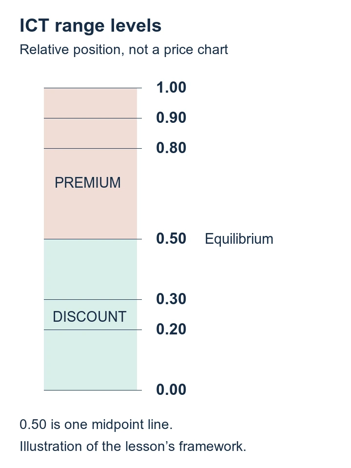
The reading rule he attaches is simple: the middle of the range, which he calls equilibrium, divides the two halves (33:15). Everything north of it is the premium PD arrays and everything from equilibrium down to the zero level is the discount PD arrays (33:36). He adds his own preferences at the extremes: the deepest discount he works with is 0.20 and he does not like to see anything less than that (34:32), 0.80 is deep premium and 0.90 is very expensive premium (34:45), and he says he does not like taking new longs at those levels or new shorts down in the deep discount (34:50).
He then uses the tool to make the location argument general. On the weekly chart, after applying the range he points out that a small bullish order block did not produce a new higher high (which he attributes to price already sitting in the premium side of the monthly range (35:25)) and concludes that bullish order blocks up in premium are not going to be as favourable as the ones down in the discount (35:34). In his interpretation, the algorithm lets price get down into a discount so larger participants can add to longs, and then price expands into a premium (35:48).
On the daily chart he makes the same point twice over. Order blocks inside the discount spectrum get responses, while premium-side order blocks produced buying opportunities he calls small pops that were not as strong as they would be lower in the spectrum (37:21). In the premium half he says bearish order blocks carry a lot of influence on price, and in the discount half a bearish order block does nothing to hold price because the algorithm keeps pressing through (37:56), which is exactly what he says he wants to see: bearish order blocks or up candles before down moves being broken like potential resistance giving way, with every down candle providing support (38:05).
ICT swing trading horizons and four-hour refinement
He draws the distinction repeatedly. Swing trading, he says, takes several days, in his words, not overnight and not intraday, which is why he gives a time horizon of two weeks or longer, and preferably about two weeks to a month, as when these trades usually play out (30:09). He also says the four-hour chart is enough on its own for this style: you can reduce the levels to a smaller timeframe to keep risk small (31:01), check a chart a couple of times a day, and if you are away from the desk intraday you can simply trade off the four-hour chart, an hour before the kill zones is what he suggests for a check-in (31:17).
He also tells students how to rehearse the method: go through your charts, note all of the discount arrays, and look for the buying opportunities that put you in sync with what you saw on the monthly, the weekly and the daily, then reduce to the four-hour to refine and keep risk small (30:48). And he attaches a warning about what the framework is not: if the structure is not behaving the way he describes, you cannot simply take an order block or buy an old low once it has been traded below and assume you have a swing trade (38:37), because swing trades in his telling are by definition very rule-based and not ambiguous, whereas day trades can flip back and forth on a noisy timeframe (38:48). His explanation for why these levels matter when they arrive is that there are not many monthly, weekly and daily levels, so a great many participants are waiting for the same ones, which he says is why they are so sensitive (39:06). He also says that if you watch and wait for these levels when they occur, it is hard not to make money doing this (39:37).
What the ICT swing lesson does not establish
This is a historical chart lesson. The transcript records the speaker’s descriptions, and the chart images were not independently reviewed for this article. The text alone does not establish actual entries, fills, position sizes, costs or account results, so it cannot verify the silver sequence as an executed trade.
Several of the specific figures are his recollection rather than documentation, and he says so himself at one point. The level he calls 15.60 comes from a candle high the caption track records as 15.56, and seconds later he concedes the number is approximate: the track reads “we are having 611 here” at that moment, and he adds that 15.80 could have been used instead (11:51). The low of the range he says he sticks at 1,400 (12:08). The low he later recalls as the bottom is 1,566 while the 1,600 area is the level he says he wanted to buy (25:21); the area reached is given as 1,797 to 1,800 with 1,802 as his remembered intraday Friday high (25:49); and the forward levels survive in the captions only as “the 19 20s and 22s”, which is not precise enough to restate as a price (29:12). The ten thousand dollars figure is presented as profit potential rather than a realised result, and it is not accompanied by a position size, a stop, a fee or a statement (39:37). The claims that these levels are what everyone is waiting for, and that watching them makes it hard not to make money, are his interpretations and are labelled as such above rather than treated as findings.
This summary follows the lesson’s automatic captions, not an independent review of its chart images or trade executions. Captions can mishear prices and terminology; ambiguous figures above are not actionable price levels.