
Key takeaways
This is the recording that identifies itself as the January 2017 long term analysis lesson 1.1, on macro analysis, and names its subject as quarterly shifts and what the transcription renders as IPTA data ranges — the Interbank Price Delivery Algorithm range 0:21.
Read the full summary
This is the recording that identifies itself as the January 2017 long term analysis lesson 1.1, on macro analysis, and names its subject as quarterly shifts and what the transcription renders as IPTA data ranges — the Interbank Price Delivery Algorithm range 0:21. His premise is stated before anything else: the market is, in his words, 100% engineered and controlled to the very pip, and the reason he takes that view is that he says he has called specific levels to the pip as exits and targets many times 4:06. From there he describes a market structure shift that recurs every three to four months across asset classes, driven by the need to generate fresh interest and urgency 5:02. The method he teaches is mechanical: put a vertical line on the first trading day of the most recently closed month, then look back 60, 40 and 20 trading days on the left for institutional order flow and reference points, and cast the same 20/40/60 windows forward to the right, because he says the algorithm reaches back about three months of data and the common denominator is always a 60-day reference 22:47. A second strand compares a traded currency against a benchmark, listing accumulation and distribution combinations based on which of the two makes a higher or lower high 9:57. Everything is applied to the daily chart, and he caps the expected wait for the next setup at roughly 60 trading days, a horizon he says is too long for his own preferences 37:34. The recording draws no charts of its own for the viewer to check: the diagrams he narrates are his slides, and no price, order, fill or result is established anywhere in it.
How we researched this article
BestProps used document-based research from primary firm sources, checked September 24, 2026. The complete source list, scope, limitations, and commercial-state record appear near the end of this article.
What This Recording Is
He introduces the material as the January 2017 ICT mentorship long term analysis lesson 1.1 and describes it as macro analysis, with the topic named as quarterly shifts and the data ranges of the algorithm he refers to as IPTA 0:21. That acronym has a specific meaning in the lesson: he calls it the Interbank Price Delivery Algorithm and says it works inside predefined data ranges set at the central bank level, that price is allowed to move to a predetermined range for the day, and that occasionally things happen which send price outside it 4:06. The value of knowing those ranges, he says, is that the trader can carry a predetermined idea of where the algorithm will do its work 4:43.
His framing sentence is worth quoting because the rest of the lesson is built on it. If there is an algorithm, he says, and the trader believes there is an automated price delivery engine providing efficiency in the delivery of price at every potential price available per asset, then the questions worth asking are where it pulls its information from, which dates, which ranges and which specific highs and lows it reaches for as reference points 0:39. He notes the teaching is aimed at foreign exchange but claims the effect of a quarterly market shift is universal across asset classes 1:42.
He spends the opening minutes arguing against randomness, and it is an argument rather than a demonstration. If markets were completely random, he asks, how could anyone reasonably have an edge, and he describes statistics as counting the odds of something already happening and attributing it to a future unseen guarantee 1:56. His conclusion is that a market which is completely random would be uninteresting to him because he would have no trust that any prognostication could fulfil a profitable condition 2:26. The evidence he offers for control is his own reported precision, and the claim that being able to repeat that through the year is what proves there is zero randomness 3:16. There is no verified track record, price series or third-party confirmation in the recording, so the claim stands as his assertion about his own forecasting rather than something the source establishes.
A sourcing note belongs here because it changes what can be claimed. The transcript used for this rewrite is automatic local speech-to-text of the recording’s own audio (Whisper large-v3-turbo), not human-verified captions, and the download passed its integrity checks: the decoded audio is complete against the listed duration, it ran to 3,308.2 seconds against a listing of 3,309, and no segment was flagged low-confidence. The automatic transcription systematically renders the algorithm’s name as IPTA in the transcript and IPA in the written text file; the standard term, and the one the surrounding explanation of an Interbank Price Delivery Algorithm supports, is IPDA, so IPDA is used here with the discrepancy recorded rather than silently corrected.
The Quarterly Shift He Describes
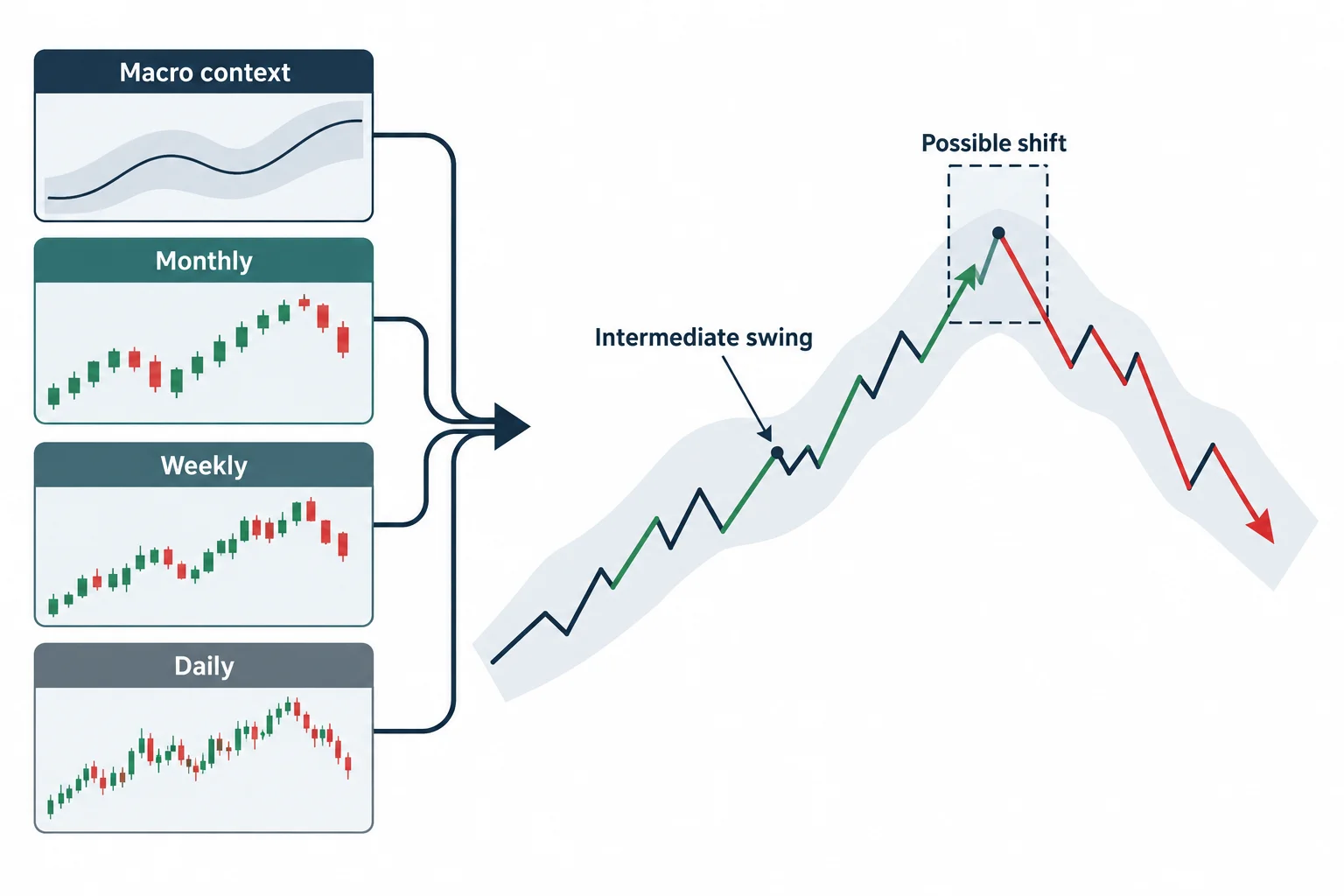
The reason for the shift, as he explains it, is new interest. He says a market structure shift takes place every three to four months, that this is universal rather than specific to forex, and that it happens because the market has to generate new interest and a new sense of urgency, with a missed opportunity being a lost opportunity in many traders’ eyes 5:02. He offers the mechanism as gyration: what was a directional movement over the last months may not be true for the coming two to four months 5:36. From that he draws a counsel rather than a signal — always look at price on a macro level, meaning monthly, weekly and daily, and learn to anticipate intermediate price swings 5:53.
What he says the trader gains is specifically about surviving long holdings. If the idea of intermediate-term retracements on higher timeframes is understood, he argues, the deep retracement that long-term position trading sometimes demands becomes easier to weather, and the trader stops treating a position as something to hold forever: part of it can be taken off, the retracement waited out, and the position added back to capitalise on the next move 5:53. He is careful about what the retracement looks like in practice: in a strong uptrend the trader may see little retracement and instead a consolidation or trading range where new longs are capitalised, and sometimes the market simply takes out a short-term low on the daily chart and then sends price higher, which would be the extent of it 7:35.
He says there is always some intermediate-term play to trade every three to four months in every asset class, and advises looking at a market that may be moving into a new uptrend or downtrend stage, which also aligns the trader with longer-term trends 8:13. On the calendar mechanics he is casual: he demonstrates a year divided on quarterly lines but says the viewer can simply put a vertical line at the beginning of the most recent past month and do the same exercise, whenever they happen to be studying 21:48. The January-to-January division he shows is treated as an anticipated quarterly shift whose truth is not known in advance — his words are that they do not know it will be true, which is precisely why the calibration step exists 22:08.
Buy and Sell Programs, Underlying and Benchmark
Before the calibration procedure he sets out what he is trying to imitate. If the trader can focus on what smart money is doing with its money and how it allocates funds into the marketplace, and mimic those characteristics, his hope is that the outcome is high-probability conditions 8:42. A buy program is defined as the market going through a series of consecutive up days, sessions or whatever the relevant timeframe is — he says a buy program is visible on an hourly chart, a four-hour chart, a daily, weekly or monthly chart alike 9:00. The trading timeframe for this month is primarily the daily chart, so anticipating a buy program means expecting a series of up days, which he says could last as long as several months, though a few up days on the daily chart still counts if price is reaching for liquidity above recent highs 9:28.
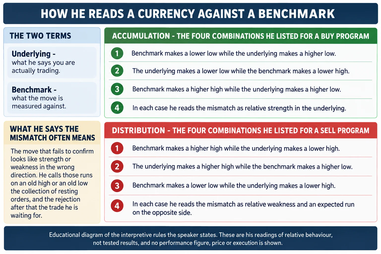
The comparison he uses is between the underlying and the benchmark, and he defines both plainly: the underlying is what the trader is actually trading, and the benchmark is what the potential manipulation, or its absence, is measured against 10:31. He flags that the lecture deals with forex first and says commodities, stocks and interest rate markets will be covered in the same venue later, deliberately keeping one asset class at a time to avoid confusing the student 9:57. He then stresses the timeframe restriction: this analysis is relative to the daily chart only, nothing less 15:53.
For a buy program he lists the accumulation combinations he reads on the daily chart. He does not label the buy-side list with a count, and three combinations are enumerated rather than four. In one, the benchmark makes a lower low while the underlying makes a higher low, which he calls strong buying pressure under the underlying and relative strength, so he would expect upside movement 10:52. In another, the underlying makes a lower low while the benchmark makes a lower high, which he says applies to inversely correlated benchmarks, and his example is the pound against the dollar going under an old low to scoop up sell-side liquidity, after which he would anticipate a turtle soup scenario on the daily chart 11:25. A third is the benchmark making a higher high while the underlying makes a higher low: in his example the dollar makes the higher high, which looks like relative strength for the dollar, while the pound-dollar makes a higher low where he says it should have made a lower low, so he reads the relative strength as being on the buy side of the pair 11:48. He adds the case of a move above an old high that takes the buy stops and then rejects, which he says would be read as a turtle soup sell on the daily 12:28.
The sell side is presented as the mirror. The benchmark makes a higher high while the underlying makes a lower high, which he describes as a sell program showing heavy distribution — his example is the dollar index making the higher high while the dollar-yen makes the lower high 13:47. Then the underlying makes a higher high while the benchmark makes a higher low, which he reads as the underlying reaching above an old high for buy-side liquidity on a turtle soup while the benchmark fails to make a lower low, so the underlying strength sits in the benchmark 14:13. The last is the benchmark making a lower low while the underlying makes a lower high: his example is the dollar index breaking a previous low to accumulate the sell stops below an old low, while the pound is unwilling to make a higher high because it is already booked with shorts and heavily under distribution 14:49. On the sell side he does describe a count, saying he will look at the four conditions he uses for a sell program, but the walkthrough itself enumerates three combinations and then explains what each implies, so the fourth condition he refers to is not separately stated in the audio 13:32. The sell side is presented as the mirror. He remarks himself that the passage was probably a little confusing and gives replacement examples, and says the rules are as explained 15:53.
One clarification in that second pass is worth keeping because it is where he defines the correlation assumption. He says the dollar-Swiss is closely correlated to the dollar index, and so is dollar-CAD when oil is not an issue, and dollar-yen is naturally positively correlated to the dollar index as well, whereas the euro-dollar and the dollar index are inversely correlated, so whatever the euro-dollar does he expects the opposite in the dollar index 17:35.
The Look Back: 60, 40 and 20 Trading Days
The procedural core of the lesson starts here. The trader takes the most recent past month, uses the first trading day of it, puts a vertical line on the chart, and then looks back to the left 60 trading days, 40 trading days and 20 trading days 22:47. His reason for those three parameters is that the algorithm will reach back about three trading months worth of data, which he calls the average, while conceding there are other times when it goes into further ranges; for the lesson he wants only the most salient points of reference on the daily chart 22:55. The detail he repeats is that these are trading days, not calendar days 23:40.
Inside those ranges he says the trader identifies institutional order flow — what the market was doing from 60 days ago up to the vertical line — and then recent institutional reference points 23:44. His list of what to mark is specific: an old price high and an old price low, looking for a potential liquidity pool resting above a high, or rejection blocks where price moved above the bodies of the candles for a potential sell-off, or below an old low with long wicks where the candle bodies might house sell-side liquidity 24:24. He adds sell stops below an old low where the lows do not carry many wicks, then bearish and bullish order blocks within the last 60 days, and specifically around the last 40 and the last 20 days, and fair value gaps and liquidity voids as well 24:47.
He works the idea with a concrete date. Speaking on 6 January 2017, he says he would use 1 December 2016 as the beginning reference point, put the vertical line on the first trading day of December, and then look 60, 40 and 20 trading days to the left of it, asking across those three months where the high is and where the low is 25:30. The bias rule that follows is stated as a rule: if the market has been trading higher he frames everything off the market low, and if it has been trading lower he frames everything off the market high 26:17. The judgement he is asking for is over the last 60 trading days at the maximum — was the institutional order flow collectively higher or collectively lower — and he accepts that sometimes it will look like a rather large trading range, which he says is still workable 26:46.
The calibration step is the part he stresses. Rather than leaving the line on an arbitrary month start, the trader moves it onto the significant intermediate-term low or high that formed in the last 60 trading days, whichever is obvious, so that the line is anchored to a previous market structure shift and to the structure that is in place now 27:10. His justification is consistency with the algorithm: if the trader believes the algorithm is systematic and methodical, working on data ranges and using calendar dates, then it has to reference how far back to look, and that is a numerical reference point the trader can calibrate to 28:19.
He then walks the dollar index through it. Anchored at 1 December 2015, the last 60 trading days to the left showed the market trading higher from around an October 2015 intermediate-term low, creating a short-term or intermediate-term high around 1 December; the last 40 trading days to the left showed a consolidation and then one more expansion higher; and the last 20 trading days showed the market simply pressing higher, so in his reading institutional order flow was bullish 29:25. From that he derives where the liquidity sits: because the market has already traded higher, the resting liquidity is below the marketplace, right beneath that October low 30:03. After the vertical line, price trades lower, and once the market structure starts to break down with the key low broken, he says any retracement or movement higher should be read as anticipating a move lower, and he expects a measure of bearishness on the dollar index after December 2015, possibly sideways consolidation 30:57.
One aside clarifies the scope of the exercise. He says he does not care about the long, long-term trend at that moment: the purpose is the quarterly shift and the context it supplies for framing position trades, and he notes that the higher-timeframe charts are not always in big long-term trends — a larger range can look dynamic on an hourly or 15-minute chart while remaining a well-defined range on the higher timeframe 31:39. Where the framework then points is at institutional reference points: price drawn down to what he calls a logical level rather than a random one, a level where the market would want to absorb liquidity or engineer new liquidity 33:17.
The Cast Forward
Once the look back is done — the ranges defined, institutional order flow identified and the reference points listed — he describes the cast forward, which uses the same parameters in the opposite direction, anticipating the next market shift in twenty to sixty trading days 34:49. The arithmetic he gives is simple and worth stating exactly: if a market structure shift is seen within the last 40 days to the left of where the trader is now, the cast forward is 40 more days, because the reference point is always 60 days 35:26. As stated in the recording the two parts do not quite close: a shift 40 days ago plus 40 days forward would put the next shift about 80 days out, while his own justification is that the reference is always 60 days. He repeats the other case — a cast forward of 40 days when the last shift was 20 days ago, which does total 60 — and states the common denominator twice: it is always a 60-day range, and the exercise continues until the extreme of the projected three-month limit 36:03. The discrepancy is in the source rather than in this summary, and the practical window he states elsewhere is the one worth keeping: the next shift is expected somewhere inside twenty to sixty trading days.
Applied to the dollar index example, that produces a calendar first trading day at 1 December 2015, a 20-day, 40-day and 60-day range to the left of it, and a future data range to the right within which the algorithm would be expected to shift 36:40. Because the market structure had broken down by the delineated low, he says the anticipation is a move lower to fill a potential liquidity void inside the 60-day window to the right 37:34. That window carries a blunt practical consequence, and he states it against himself: a daily-chart setup may be up to 60 trading days away, which is why he says he is not a heavy position trader and does not have the capacity to wait that long, while noting it may suit others, and that the same context can still be used for daily bias, short-term setups and long-term objectives 38:27.
He applies it to the euro-dollar next, on the inverse-correlation assumption: expecting bearishness in the dollar index means expecting bullishness in the euro-dollar, so the same 20, 40 and 60 days are added to the right of the same 1 December 2015 line 38:47. His practical note here is about the platform: on MT4 he suggests a trend line anchored to the vertical line, dragged out to the right, released and re-grabbed to extend it until the readout says 20, 40 or 60, at which point the delineations for the data range are set 39:17. He then points at what he calls the high on the euro-dollar falling directly at the 60-day data range and says the range nails the very high, before restating the logic that if the behaviour is not random and is manipulated and controlled, it should repeat and be measurable 39:55.
The pattern he describes as recurring is a market structure break in one direction followed by a run the other way that closes a void. In the dollar index example, after the structure broke below the delineated low, all the successive higher highs inside the 60-day window to the right of 1 December 2015 were, in his reading, nothing more than retracements closing in the liquidity void 43:20. The reason he treats it as accumulation rather than genuine bullishness is the cross-check against the related currency: the euro-dollar lows inside the same 20, 40 and 60-day windows to the right were higher, which he reads as the underlying failing to make a lower low while the benchmark makes higher highs, and therefore as accumulation 44:16. He is explicit that the higher highs would look like bullishness every time a new high formed, and that in his account all it was doing was inching up to close the void 44:58.
He adds a second marker lat