
Key takeaways
ICT Mentorship Core Content Month 05 Lesson 2.2 presents IPDA, the Interbank Price Delivery Algorithm, as a study framework using nested 20, 40, and 60 trading-day lookback and forward windows on the March 2017 Australian dollar futures contract.
Read the full summary
ICT Mentorship Core Content Month 05 Lesson 2.2 presents IPDA, the Interbank Price Delivery Algorithm, as a study framework using nested 20, 40, and 60 trading-day lookback and forward windows on the March 2017 Australian dollar futures contract. Traders identify the most obvious bullish or bearish market-structure shift from roughly the prior three months, roll the anchor back to the first trading day of that month, then count forward 20, 40, and 60 days while marking each window’s highest high, lowest low, buy stops above highs, sell stops below lows, gaps, fair value gaps, liquidity voids, and equilibrium midpoint. The case study anchors to a quarterly bearish shift in November 2016, with the 40-day window containing a low near 71.50 that preceded a significant move. These windows are not turn-date forecasts, and direction must come from higher-time-frame analysis. If liquidity above and below the prior 60-day range has already been cleared, the method looks outside that range for the next high and low. ICT argues that finite software reference data and habitual stop placement explain the 20, 40, and 60-day ranges, but the recording provides no statistical test, sample size, or performance data for a controlling algorithm. His open-interest interpretation treats a roughly 15% or larger decline while price moves sideways as bullish and maps open-interest peaks near swing highs to central-bank sell programs, although exchange data does not identify a specific counterparty. Students are instructed to journal dated charts and track how long anticipated levels take to be reached, with waits ranging from several days to two weeks, making the framework a forward observation routine rather than a tested trading system.
How we researched this article
BestProps used document-based research from primary firm sources, checked September 24, 2026. The complete source list, scope, limitations, and commercial-state record appear near the end of this article.
In ICT Mentorship Core Content – Month 05 – Using IPDA Data Ranges, the speaker spends two hours on one idea: that price is drawn to reference points which can be located in advance by looking back, and forward, in fixed windows of trading days. This article follows the recording in order and links each substantive point to the passage it comes from.
Three limits apply throughout. The charts he is walking through are not visible in an audio transcript, so nothing here asserts a specific swing value, price level or fill as verified – the numbers that appear are the ones he states aloud. Second, the causal framework he builds around an algorithm and central-bank liquidity is his explanation, and the recording contains no test, sample size or performance data behind it. Third, the transcript is automatic speech-to-text of the audio rather than human-checked captions, so the acronym and a handful of other renderings are flagged near the end rather than silently corrected.
Starting the ICT IPDA Data Range Lesson
He opens by announcing an IPDA data-range example on the Australian dollar, and immediately turns to a practice point rather than a technique. He says he wants students watching the levels on the charts he shares, and to notice how long price takes to reach them (0:00:06, 0:00:11).
The theme he returns to repeatedly is the gap between a hindsight example and an observation made in advance. He calls the waiting period the main point of the lesson, saying a trader has to learn to wait for these things to unfold (0:02:45), and he describes how long that wait actually is in trading days – three days, four days, two weeks (0:04:11). He is unusually candid about his own temperament here: he says he is not really a patient person at all, describes himself as very impatient, and gives that as the reason he does not do long-term position trading (0:03:00).
The practical instruction is a journalling routine. He tells students to copy or print the charts, keep a running log, put them in a three-ring binder with dates punched in (0:05:30), and hold him to the standard that if the observations were sound they should be evidenced in the record (0:03:27). He names hindsight chart cherry-picking as a problem directly, saying that when he flags a point in advance it is not a trophy being shown in passing (0:10:05).
He then sets up the instrument. The example runs on the March 2017 Australian dollar futures contract, and he argues that a forex trader should study the underlying futures chart because spot foreign exchange does not give you volume (0:48:58, 0:08:11). He says he is showing a little under six months of that contract, only because beyond that the chart becomes patchy as the December contract expired (0:08:27).
How Beginners Can Use ICT IPDA Data Ranges
He resets the exercise to the simplest possible version: if a brand-new trader sat down with the Australian dollar chart today, how would they find where the IPDA data ranges are (0:09:26)? His answer is to start from today’s candle and go back through the last three months (0:09:54).
He anticipates the objection about hindsight before making his point. He quotes the imagined critic saying here we go again, and agrees that it is a hindsight thing – then says students need to understand what the ranges are actually meant to do (0:10:05). What they are not, he says, is a countdown: students assume it will call the high and low 20, 40 and 60 days away, and he says that is not what happens, though sometimes it can and does (0:10:18).
The question he says the ranges are meant to answer is a specific one traders keep asking him: when looking for an order block to buy from or sell into, or an area of buy or sell stops, which one will price go after, and how do you know it will not simply run through an old high (0:10:34)?
Anchoring the ICT IPDA Data Range Framework
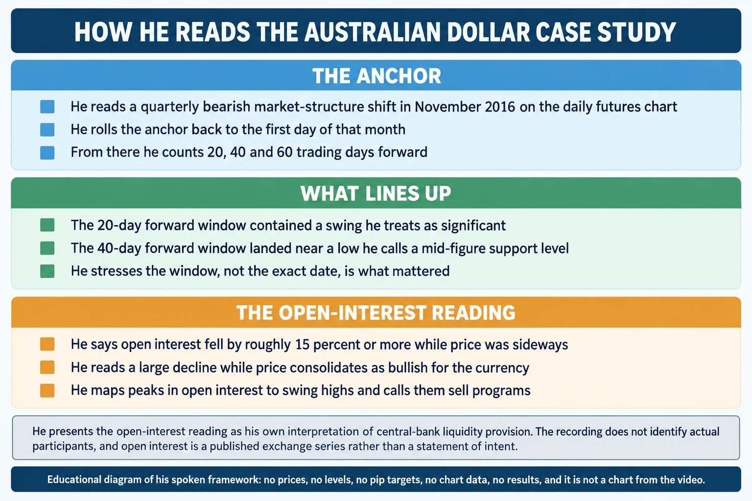
The starting point of the whole method is finding the most obvious market-structure shift. He says the most recent one in the last three months occurred in November, and flags a market shift there on the futures chart (0:09:54, 0:09:54). He reads it as displacement by large players, calling it a quarterly market shift and describing it as the most obvious one over the last three to six months (0:11:43, 0:11:57).
He then generalises: something like this occurs roughly every three months, either a sell-off that creates a high or a low from which price starts to rally, and he wants students looking at their charts to anticipate finding it in hindsight (0:12:26). He notes the shift in his example was a high being made, with a low broken, and that it involved taking out an area of equal highs and piercing above it to take out the buy-stop liquidity pool – which he offers as the basis of the structure shift (0:14:50, 0:14:50).
This is the step people skip, and he is emphatic about it. Once the shift is identified, the trader must roll back to the beginning of the month it occurred in, because a basis point is needed – where did it all begin (0:39:07, 0:15:50)? He says the shift occurred in the second week of November and they now calibrate to the first of that month (0:39:07).
He also warns against over-selecting. If a student picks out a smaller, more convenient move and calls it the obvious one, he says they are doing too much anticipation: the requirement is the most recent obvious bullish or bearish move, which may mean going back three months (0:16:12). His practical shortcut for the eye is to divide the daily chart into quarters with lines at March, June, September and December (0:16:33).
Understanding the 20 40 and 60 Day IPDA Ranges
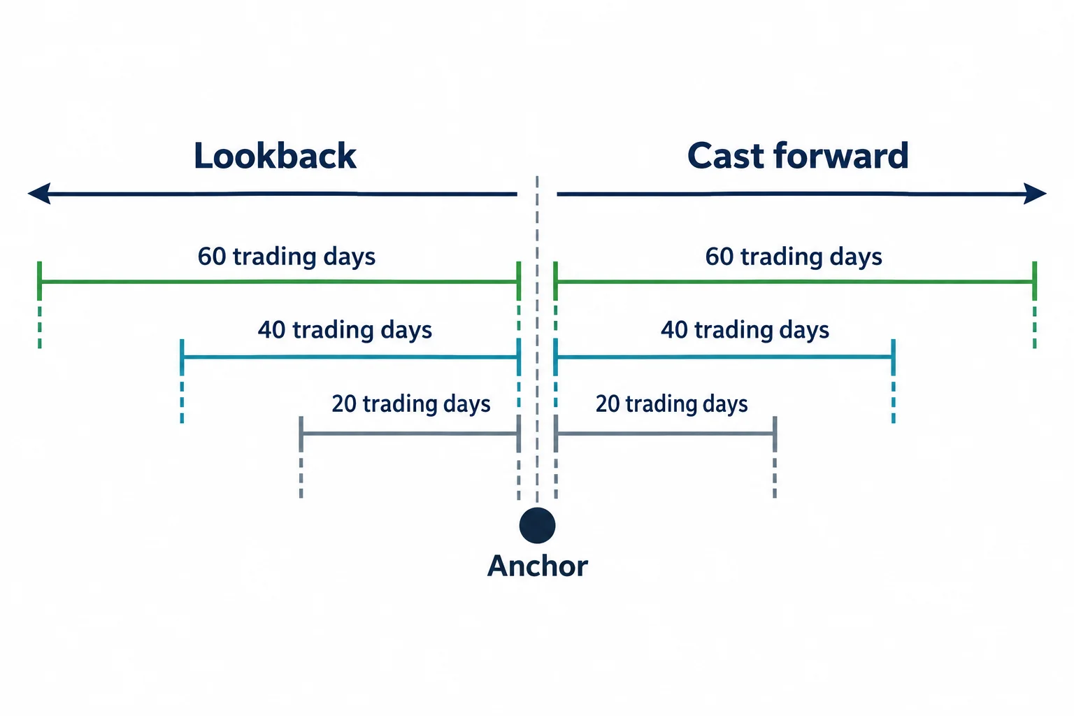
The ranges themselves are stated plainly: a 20-day lookback with the same window cast forward, then a 40-day, then a 60-day (0:13:22). From the first day of the anchor month he counts out 20 trading days forward, with the option of using an even more obvious nearby point if it genuinely is the obvious one (0:15:50). He later describes looking back 20 trading days from a point 40 days forward, so the windows are nested and reusable rather than fixed forever (0:42:35, 0:45:00).
Inside each window he lists what to find. The highest high and the lowest low come first, and he explains why in terms of where traders put stops: above the old high there will be buy stops, below the old low there will be sell stops, and that is where he says the algorithm looks for liquidity (0:27:56, 0:28:02). Then gaps and fair value gaps – places where price has not been efficiently delivered – and the liquidity voids where price has only been delivered one way and has to come back to balance (0:17:14, 0:17:21). Then equilibrium, which he ties to the midpoint of the range and to the optimal-trade-entry idea (0:17:40, 0:17:40).
He adds the case where both sides have already been cleared. If everything above and below the highs and lows of the last 60 days has been wiped out, there are no stops left in the window and the market has to create new expansion, so the trader looks for the next high and low outside that range (0:33:08).
Why ICT Uses These IPDA Data Ranges
The reason the lookbacks are 20, 40 and 60 days is not presented as a statistical finding. It is an argument from how software works. He asks how a computer program could know where everyone’s stop is (0:25:07), and answers that it needs a range of data to work from (0:13:22).
The part of that argument worth keeping is his stated reason the program cannot simply read order books. He says the algorithm does not see orders, and that individual traders are dynamic – stops get moved, trades get collapsed, so no book of orders exists to be read (0:27:08, 0:30:51). The standardised substitute, in his account, is human habit: traders put sell stops below an old low and buy stops above an old high, so those levels are where price is drawn (0:30:51).
Around that sits a much larger claim, and it should be flagged as one. He says price is not random, that there is an algorithm controlling it running on a script that refers to specific data points it returns to repeatedly, that the market was once manipulated manually by people and is now done more efficiently, and that the algorithm permits price to move to a level so bank-level traders can execute there (0:13:11, 1:38:58). He also says the algorithm looks back 60 days to find the highest high and lowest low (0:17:14). The existence of a controlling algorithm, the identity of any operator and the motives assigned to it are his framework, not findings the recording establishes.
Applying IPDA Data Ranges to the Australian Dollar
He then works the November 2016 anchor through the windows. Casting 20 days forward from the first of November, he says there is going to be a significant setup inside that window, notes that price moved up into an old low formed in October and then went into consolidation rather than making a clean shift (0:34:24, 0:34:41).
The 40-day forward window is where the example becomes concrete. He marks it as the 40 days out from the beginning of November, framed on the quarterly shift (0:35:33), and points to a low he identifies at about 71.50 on the Australian dollar, describing it as a mid-figure level happening inside that window (0:40:51, 0:40:51). He says a significant price move occurred from that level and expects the obvious response from students (0:36:43).
The most important qualification in the whole lesson sits right here, and he makes it twice. He says the point is not that the 40th day produced the lowest low, but that the low formed in proximity to the window – the turning point could have happened any time in those 40 days (0:35:47, 0:44:37). He compares the behaviour to an indicator he used to rely on, Williams percent R, which he says gave him the day before the real oversold condition many times, and says the same can happen with these ranges – a turn may occur on the 19th day or the 20th, and that is not what the trader should be relying on (0:38:04, 0:37:56, 0:38:26).
The summary of that passage is the sentence to hold onto: he is not telling students that markets turn every 20 days, every 40 days and every 60 days, but it can and will sometimes do that (0:38:50, 0:38:55). What he says the trader is actually looking for is the quarterly shift, with the range supplying the frame around it (0:39:20).
He then reuses the frame going forward: having a vertical line 40 days ahead means the trader can also count back 20 days from that future point and ask where the highs and lows are (0:42:35). In his example that count lands on the second to the last day in November, and the highest high inside it forms in mid-December at an area of equal highs, which he again treats as a resting buy-stop pool that price will seek out (0:43:26, 0:43:32, 0:43:48).
Reading Daily IPDA Data With Higher Time Frames
He is clear that the daily windows do not stand alone. He says the read is more confirmed when applied to the weekly and monthly charts, because levels just outside the 60-day window start to align with higher-time-frame references (0:33:08). In his example he points to a weekly level at 71.50 that price had tapped twice before and repelled from aggressively, and to old highs and lows whose buying and selling pressure he treats as evidence (0:48:11, 0:47:55). He also marks a bearish order block in the last week of October 2016 and describes a range that could take the pair up toward 75.70 (0:48:30, 1:08:10).
He separates the horizons carefully at this point, and the distinction is worth preserving. He says quarterly cycles and the ebb and flow of a rally and decline inside them are short-term in nature, while monthly and yearly moves are driven by real fundamentals such as interest rates (0:41:25, 0:41:31). He puts three months in perspective against a five- or ten-year trend, saying a three-month cycle is not significant at that scale and that macro fundamentals are not impacted by it, though it can be used to get in sync with them (0:41:43, 0:41:55). He also says the only fundamental he teaches is interest rates (0:42:08).
His own working horizon is stated as about three months, and he says he does not like to look beyond that, describing himself as often accurate on a four-to-six-week horizon which he calls about the half-life of the three-month cycle (0:18:18, 0:18:34, 0:18:40). He argues the horizon is useful across disciplines rather than only for position traders, naming long-term position, swing, short-term intraday and scalping (0:19:07).
Using Open Interest With ICT IPDA Data
The second half of the lesson turns on open interest, and he credits the source directly: the book he names is How I Made a Million Dollar Trading Commodities Last Year by Larry Williams, which he says was written in the 1970s and which he recommends as an essential part of a trader’s library (0:50:12, 0:49:45). He argues open interest is the most misunderstood data point in trading (0:50:32).
His base case is the same as the standard one: open interest is the total open longs and shorts in the market (0:56:57). Where he departs from the textbook framing is in who he says the counterparty is. He argues the central bank is the storehouse for price and the liquidity provider for its own currency, so open interest can be viewed as every trade the central bank is providing counterparty to (0:57:03, 0:57:33), and that a 15% or larger drop in open interest while price is sideways is bullish, because it indicates the provider no longer wants to hold the heavy short position it had built by selling to buyers (0:58:32, 0:58:44).
The technique he adds to that is mapping. He says that by matching the swing highs to the peaks in open interest, you can see where the sell programs were executed – that every peak in open interest from the low is a high, and the largest peak is where the most was sold (0:59:52). In the worked example he describes a range between roughly 77 and 74.50 through August, September and October, a false breakout above 77 in November that rejected and traded lower (0:56:07, 0:56:14), and then a decline in open interest through the sell-off which he reads as those short positions being covered (1:01:02). He points to a sharp drop in open interest in December as the central bank clearing out remaining shorts, and says the sell program was completed between the first week of November and the middle of December (1:04:11, 1:04:34), estimating the book was built from 77.50 down to 71.50 (1:04:53).
He also gives the general shape of the cycle he thinks repeats. He says every three months there is a major shift, at a support level, where a large drop in open interest accompanies the reset (0:54:21), and that banks do rapid declines specifically to take away near-term bullish sentiment before the reset (1:02:20). He explicitly acknowledges that the framework does not remove risk: asked what real risk exists if participants control price, he raises the possibility of major geopolitical shocks and points to September 11 and Brexit (0:23:33).
Two things about this section need to be kept apart. Open interest is a published exchange series, and its level and change can be checked independently. The readings he builds on top of it – that the counterparty is the central bank, that a specific peak is a specific institution’s sell program, and that the motive is to reset exposure – are his interpretations of that series, and the recording supplies no participant-level data behind them. The article reports them as his framework for that reason.
How the ICT IPDA Data Range Example Resolves
He closes the case study by describing what he expected and what he says followed. He states that he was not bearish on the Australian dollar in that period (1:06:41) and that the expectation was for price to come up into the range and potentially into the bearish order block (0:48:30). He points to the 40-day forward candle as the day price moved higher and created a down candle which he treats as a bullish order block (1:05:31,