
Key takeaways
ICT Charter Price Action Model 10 is a weekly swing framework built on two halves.
Read the full summary
ICT Charter Price Action Model 10 is a weekly swing framework built on two halves. The first half is a five-stage trade plan: preparation, opportunity discovery, trade planning, trade execution and trade management. It sets a 50-to-75-pip weekly objective, determined from 20-, 40- and 60-trading-day dealing ranges, and it times entries to a 15-minute liquidity raid during the London or New York open after a calendar event. The second half is the algorithmic-theory lecture: he treats a consolidation as a dealing range, identifies which side of it holds resting liquidity, and expects price to run the external range liquidity on one side and then deliver to the opposite side. Management rules are given explicitly – a sell limit five pips below a PD-array convergence and a buy limit five pips above it, two orders per idea with the bulk taken at 50 pips, a stop reduced 25% at half the objective and moved to breakeven at 75%, and a position-size formula with halved risk after a full-R loss. The source is automatic speech recognition of the audio, so no fill, price or outcome in it is verified here.
How we researched this article
BestProps used document-based research from primary firm sources, checked September 24, 2026. The complete source list, scope, limitations, and commercial-state record appear near the end of this article.
In ICT Charter Price Action Model 10 – Trade Plan & Algorithmic Theory, a public upload on The Inner Circle Trader channel, the model is presented as a swing-trading plan for a week rather than a single session. The video was published on 9 February 2024 and runs about twenty minutes.
Two limits shape how this should be read. The source here is automatic speech recognition of the full original audio rather than human-authored captions, so slide headings and a few terms are handled as reported speech and one repeated phrase is ambiguous. The slides, charts and order panel shown in the recording were not inspected for this article, so no level, fill, spread or result in it is confirmed here.
The five stages of plan development
The plan is laid out as five stages at 0:30: preparation, opportunity discovery, trade planning, trade execution and trade management (0:35). He also restates the model’s objective at the top of the recording as 50 to 75 pips per week on a swing-trading timeframe. Splitting analysis from execution this way is the most transferable part of the lesson; the rest is his own market interpretation.
Preparation: the calendar and the dealing range
Preparation starts with the economic calendar. He says to note every medium- and high-impact event for the markets being followed and to consider how the current market structure and those events may suggest a specific weekly profile for that week’s range (0:46, 0:50).
The range itself comes from three lookbacks. He uses 20, 40 and 60 trading days, excluding Sundays, notes the highest high and lowest low in each, and calls the result the current dealing range (1:02, 1:16, 1:22). Inside it he asks where price is likely to trade next: below which old low, above which old high (1:30, 1:35).
At 1:39 the automatic transcript renders the term as “PDRA” when describing what he looks for in the direction of the weekly range bias, then later uses “PD array” in the management rules. The expansion is most likely price delivery array – the same phrase used in the later rule about a PD-array convergence – but the slides were not inspected, so the exact wording is flagged here rather than asserted.
He then ties the two pieces together: the expectation is that price moves to a delivery array supporting the weekly bias on a day and news release found on the calendar for the current or next trading week, and he calls that volatility injection what he waits for (1:45, 1:54).
Opportunity discovery: the 50-to-75-pip range
Opportunity discovery looks for a 50-to-75-pip range that would allow a run to buy-side liquidity when bullish institutional order flow is present, or target sell-side liquidity when bearish order flow is present (2:03, 2:10). He states his own preference plainly: he takes the bulk of the weekly objective at 50 pips and treats the 75 as a remainder (2:33, 2:39).
He also describes the structure as two orders: one taking 50 pips as the objective, and a second that may not reach 75 but that he calls the best case for the model (3:05, 3:17). Nothing in the recording establishes that either objective was reached in any particular week.
Trade planning: convergence, then the injection
For a decline he says to look for a convergence of manipulation and price opposite to the trade bias at a time the calendar suggests a volatility injection, and to short premium buy-side liquidity pools; for a rally, the mirror: buy discount sell-side liquidity pools (3:22, 3:39, 3:51).
Execution narrows the timeframe and the clock. When bearish he anticipates a 15-minute buy-side liquidity pool raid forming from a retracement higher during the London open and/or New York open kill zones; when bullish, the reverse – a sell-side pool raid from a retracement lower (3:59, 4:10, 4:17). Kill zone, liquidity pool, PD array and institutional order flow are his terminology and are assumed here to be understood from his other material; this session does not define them.
Management: the stated rules
The management section is unusually explicit, so it is worth reproducing closely. Entries are limit orders on a demo account: for a short, a sell limit at the PD-array convergence minus five pips; for a long, a buy limit at the convergence plus five pips (4:29, 4:38, 4:47). Two orders carry the idea: the first takes 50 pips, the second anything above 50 and up to 75 (5:05, 5:12). If the 75-pip objective is captured the second order is closed by limit and he waits for another opportunity (5:21).
- Two orders express one trade idea (5:18).
- First objective 50 pips on a single position (5:05).
- Second order for anything above 50 and up to 75 pips (5:12).
- Stop-loss can be reduced by 25% once 50% of the expected objective is in profit (5:58).
- Stop-loss can be moved to breakeven once 75% of the expected objective is in profit (6:05).
- Round position size down (7:22).
These are stated as model rules. A transcript cannot establish how a stop actually behaved, what spread and slippage were applied, whether a limit filled, or how any week resolved, and none of that is asserted here.
Position sizing and the adaptive risk rules
The sizing formula he gives is position size equals account equity times the chosen risk percentage divided by the stop loss in pips, and he defines each term, noting that the stop distance is the difference between entry price and stop (6:16, 6:26, 6:37).
His worked example uses a $10,000 hypothetical account and 1% risk, which is $100, against a 20-pip stop (6:48, 6:55). He runs the same numbers three ways. At $0.10 per pip on micro lots the 20-pip stop is $2, so the $100 budget allows 50 micro lots; at $1 per pip on mini lots it is $20, allowing five mini lots; and at $10 per pip on a standard lot the 20-pip stop is $200, which he says is immediately over the 1% budget, so standard lots simply do not apply (7:02, 7:36, 8:11, 8:25). He tells the viewer to always round down at each step (7:22).
Two risk rules sit on top of that. If a demo trade loses the full chosen risk percentage, he says to drop that percentage by 50% and restore it once half the loss is recovered; and if a reduced-risk trade also loses, to halve again until the previous loss is half recovered (8:32, 8:37, 8:45). Separately, after five consecutive winning trades he says to drop the risk percentage by 50%, on the reasoning that a loss is likely eventually and that this builds equity levelling and reduces the chance of a large drawdown (8:55, 8:59). His stated aim is a smooth equity curve ascending in stair steps rather than a jagged or deep decline (9:06).
These are presented as discretionary rules, and the recording supplies no backtest or comparative figures for them. The five-wins rule in particular is a counter-trend risk adjustment rather than a tested property of the model.
Dealing ranges and external range liquidity
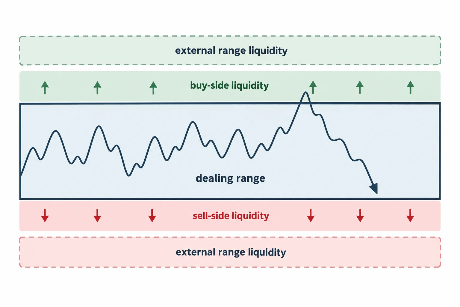
The second half is the algorithmic-theory lecture. He frames the model as weekly range expansion specific to day of week, using external range liquidity in the direction of that expansion (9:28, 9:34, 9:39, 9:46).
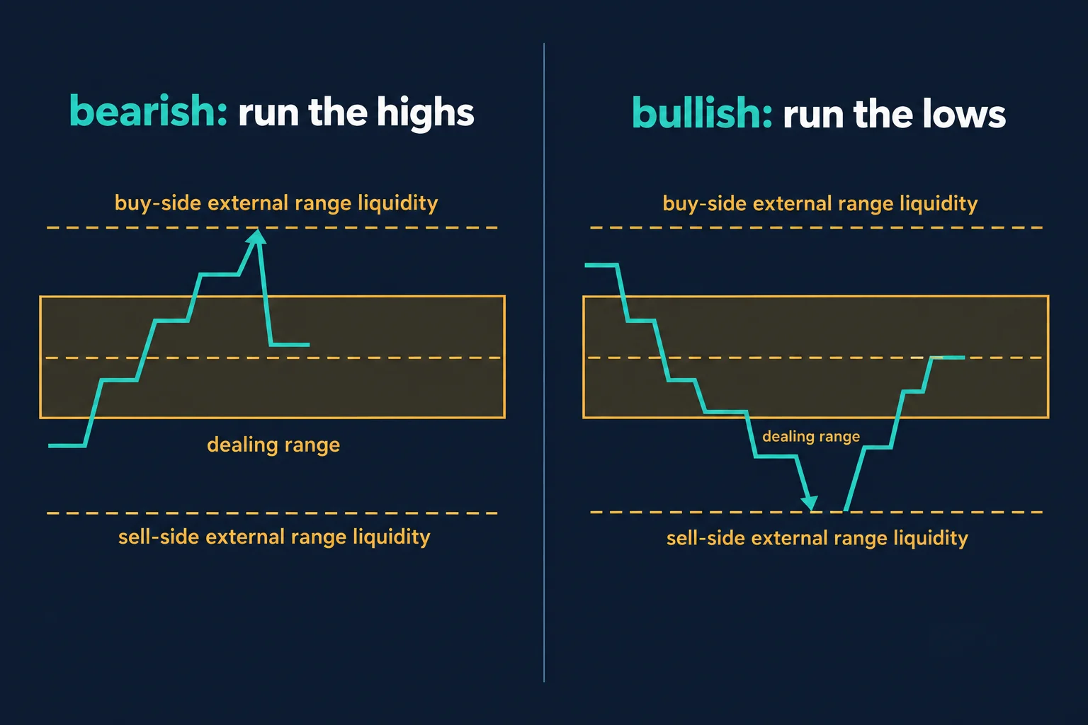
In the bearish example he points at a high, says buy-side liquidity rests right above it, describes that level being run, and says he looks to short there and wait for a short-term low and a discount to form with resting sell-side liquidity (10:07, 10:12, 10:15). His description is mechanical about who is on the other side: he says he is selling into buy stops to get short and buying sell stops to cover, waiting for a short-term high to be pierced when bearish, riding down to a future short-term low, and covering from sellers below the market (10:30, 10:38, 10:58).
He then pre-empts a reasonable objection himself, which is worth noting because it is the crux of the concept. Asked whether the high-to-low span is not internal range liquidity, he agrees it is if you refer to that range, and says the liquidity he means is external to the range he is framing – the low-to-high span – and that stops from traders who shorted would rest just above the high he expects to be run (11:30, 11:37, 11:46). The definition therefore depends on which boundary the practitioner frames as the dealing range, which is a judgement call rather than a fixed rule.
Dealing ranges are also described as fractal. He says they behave like consolidations and nest inside one another, and points out a larger consolidation housing several smaller dealing ranges, with a still smaller one visible on a lower timeframe, adding that they fit together like a puzzle (15:07, 15:12, 15:18, 15:39).
He illustrates the bullish pairing on an E-mini S&P example: from a low-to-high equilibrium resting area, price trades down into a small gap that is both discount and fair value gap, he anticipates a rally, and he wants to see it run above the short-term high or rebalance the area above (12:15, 12:30, 12:39). He identifies that chart as a one-minute chart and returns to the question of how to define the range (13:12).
On that definition he offers an analogy rather than a formula: think of a dealing range as a trading range, an area the market stays inside in a roughly rectangular way, even if it does not look like a rectangle at first (13:23, 13:27). He adds that he only cares about the external side he intends to trade: when bullish, the sell-side external range liquidity below the range; liquidity above is buy-side and below is sell-side (13:45, 14:17, 14:26).
There is one reported outcome in the recording, and it is worth attributing rather than repeating as a result. He says he recorded a trade in the S&P and shared it on his own social account that week, that his entry was buying sell stops as external range liquidity below the range, and that his orders were filled at the level he had identified as the buy-side draw (14:32, 14:39, 14:46, 15:29). That is his own account of his own execution. No statement, account record or independently verifiable fill supports it, and it is not presented here as evidence the model works. He also notes he was expecting a push higher on index futures early in the week while saying explicitly that he was not claiming the closing price would be higher or lower (16:34, 16:43).
His claim about the algorithm, stated as a claim
The recording’s strongest assertion is about cause. He argues that reaching the draw is not buying pressure pushing price up or a short-covering rally caused by buy orders, but that the algorithm already knew where it wanted to go because that is where smart money would offset and distribute (17:47, 17:57, 18:10, 18:33). He also dismisses educators, books and authors who explain such moves through buying pressure as not knowing what they are talking about (17:49).
That is a contested causal claim about market microstructure, not an established fact. It is reported here because it is central to how he presents the model, and a neutral reading is available: the framework uses prior range boundaries as candidate reaction zones and targets, conditional on bias, time of day and day of week, without requiring the market to have selected a destination in advance. The recording offers no test that distinguishes the two readings.
He closes by pointing at the practical side: the pattern repeats because it is fractal across second, minute, 15-minute and hourly charts, and he estimates he looks at this setup about a dozen times a week, but that a practitioner still has to blend the measure of bias with time of day and day of week (18:12, 17:06, 19:11). His summary line is short: buy below old lows and sell to old highs when on side with the bias (20:07).
What the session does and does not establish
The plan half is concrete and reproducible as a checklist: mark the calendar, mark the 20/40/60-day extremes, choose the side with room, wait for a session kill-zone raid, use limit orders offset five pips from the convergence, split the idea across two orders at 50 and 75 pips, trim the stop at half the objective and move to breakeven at three quarters, and size from equity times risk divided by stop distance. The theory half is a set of interpretations – dealing ranges, external range liquidity, and algorithmic delivery – that the recording asserts rather than demonstrates.
What is missing is evidence. There is no win rate, no account statement, no verified fill, no backtest and no comparison against trading the same levels without the framework. The 50-to-75-pip objective, the five-wins risk reduction and the algorithmic claim are his statements, and the only reported execution is his own recollection of a trade he says he recorded.
Watch the original recording
This embedded player was loaded, opened and clicked from a BestProps page on 14 September 2026 and began playing at the recording’s own duration, so the video can be watched in place. The timestamp links above point at the passages being described.
Primary source and further reading
- The original Inner Circle Trader recording — the timestamp links above are the passages being described; the video runs about twenty minutes.[1]
- CFTC fraud advisory — commodity trading systems sold on the internet — the U.S. derivatives regulator’s warning that hypothetical results assume fills at specific prices, that stop orders may execute at a worse price or not at all, that bid/ask spreads may not be reflected in backtested or hypothetical prices, and that commissions and fees raise the break-even point.[2]
- CFTC Learn & Protect — forex frauds — the regulator’s own statement that two out of three retail foreign exchange traders lose money each quarter, and that past results do not guarantee future success, relevant to a weekly pip objective presented without a verified record.[3]
- CFTC Learn & Protect — registration and fraud checks — the reminder that there is no such thing as a risk-free trade or investment, and that markets and products should only be traded with entities registered with the CFTC or other federal or state regulators.[4]
- 17 CFR 4.41 — advertising by commodity pool operators and trading advisors — the rule requiring testimonials to be qualified as non-representative and stating that no representation is being made that any account will achieve similar profits or losses, cited because the recording’s reported execution is a single self-described trade with no accompanying record.[5]
Any ICT, SMC or third-party indicator, script, transcript, note set, spreadsheet or social summary circulating outside the publishing channel’s own upload page is unofficial and untested here. Dealing range, external and internal range liquidity, PD array, buy-side and sell-side liquidity pool, institutional order flow, kill zone and algorithmic price delivery are the speaker’s own framework and terminology. No win rate, drawdown figure, fill, position size or account result is claimed anywhere in this article.
Leveraged currency and futures trading carries substantial risk. A weekly pip objective, a halved risk percentage after a loss and a stop moved to breakeven at part of the objective all change the distribution of outcomes, and the recording’s own sizing example shows a standard-lot position breaching the stated 1% risk budget on a 20-pip stop. This article is educational commentary, does not provide individualised financial advice, and reports no outcome from any session or account.