
Key takeaways
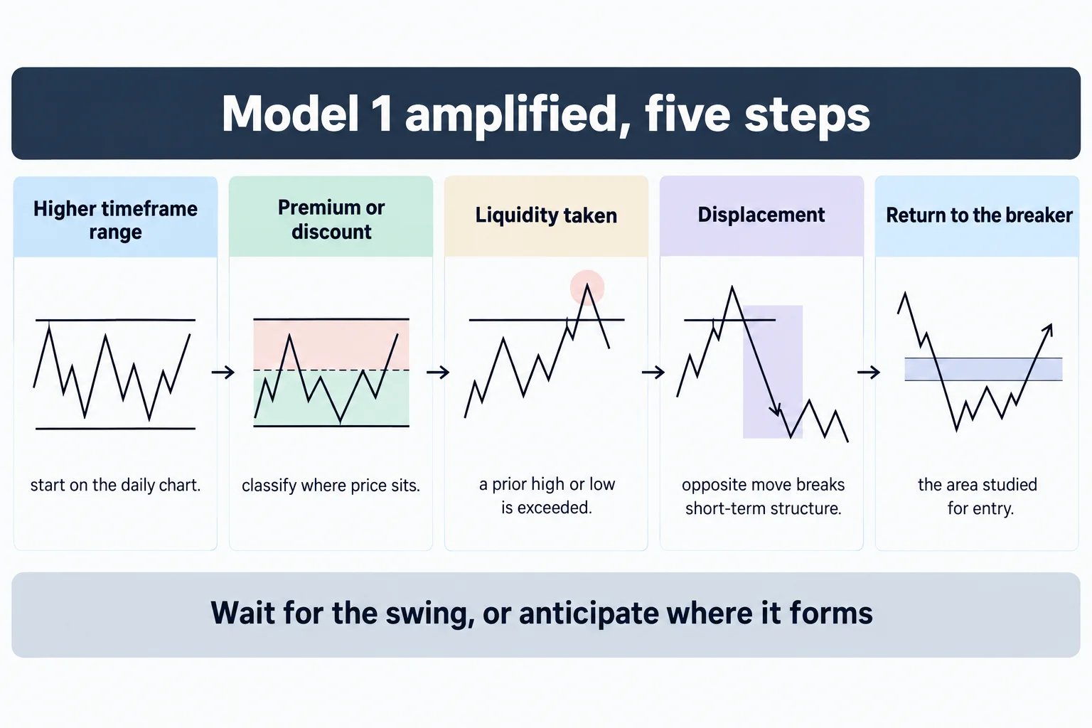
ICT Charter Price Action Model 1 \ Amplified Lecture takes the foundational model – wait for a swing high or low to form, then trade the break – and replaces the wait with anticipation.
Read the full summary
ICT Charter Price Action Model 1 \ Amplified Lecture takes the foundational model – wait for a swing high or low to form, then trade the break – and replaces the wait with anticipation. In this version the speaker starts from a higher-time-frame dealing range, classifies price as premium or discount, waits for a prior high or low to be taken, requires displacement that breaks short-term structure, and then studies the retracement back into the breaker for the entry rather than waiting for the swing point to complete. The illustrated case is a daily New Zealand dollar chart with execution on the 15-minute chart at a 62% retracement, targeted at prior daily highs. He calls the original rule a training wheel for beginners, says his own trading plan fits on the back of a business card, and states plainly that setups get stopped out. The later material also contains a compounding illustration built on an assumed 2% weekly return; that is his arithmetic on stated assumptions, not a demonstrated result, and the recording contains no audited record, sample size, costs or drawdown data.
How we researched this article
BestProps used document-based research from primary firm sources, checked September 24, 2026. The complete source list, scope, limitations, and commercial-state record appear near the end of this article.
What This Amplified Model 1 Lecture Covers
At 0:31 the recording opens with a bare welcome and moves straight into the subject. At 3:09 he says his trading plan is written on about the back of a business card, and at 3:23 that he wants it kept there. At 3:40 he states the plan in one breath: trade institutional order flow into inefficiencies on a scalping basis, primarily Monday, Tuesday or Wednesday with an occasional Thursday, exiting at external range liquidity. At 3:58 he adds that he leaves part of a position on when it is profitable so an unexpected expansion pays for the small losses.
He also pre-empts a common objection about complexity. At 1:49 he says he uses selected tools rather than every possible intermarket or overlay relationship, and at 1:56 that he does not want to give the impression a student must have everything in the model. The contrast he draws later is with an extremely long submitted trading plan.
The Foundational Rule He Says He Is Amplifying
The base version is stated at 7:35: the foundational study uses swing points, waiting for swing highs and lows to form, then buying when a swing high is broken and selling short when a swing low is broken. At 8:14 he calls that a good training wheel to start, the free beginner material rather than the finished method.
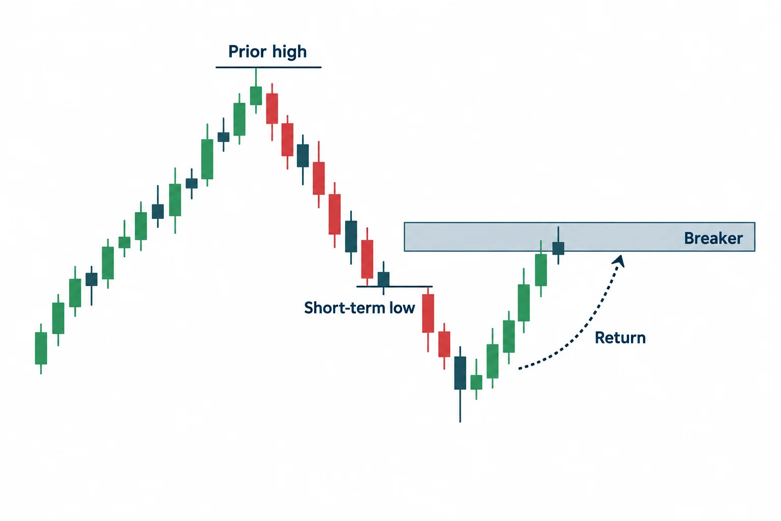
The amplified version changes the timing question rather than the direction question. At 15:00 he describes the short context as a high being run and the high being broken, then a short-term low taken out, then price trading back up into the area he calls the breaker. At 15:19 he says the swing points are not necessary because the trade is taken at the level instead of waiting for them, and at 15:25 he puts the entry band at 10 to 30 pips above the high. At 15:42 he repeats that price is traded as it returns to the breaker rather than waiting for the swing high to form, and at 15:48 gives his reason: it produces better entry points.
The bullish mirror is set out at 16:32, where he says everything is reversed below the equilibrium of the current dealing range, and at 16:36 that in discount the ideal scenario for buying starts with a prior low being violated. At 17:05 he describes the upward displacement that breaks the short-term high, and at 17:10 calls the resulting breaker the highest form of the idea.
Premium, Discount and the Dealing Range
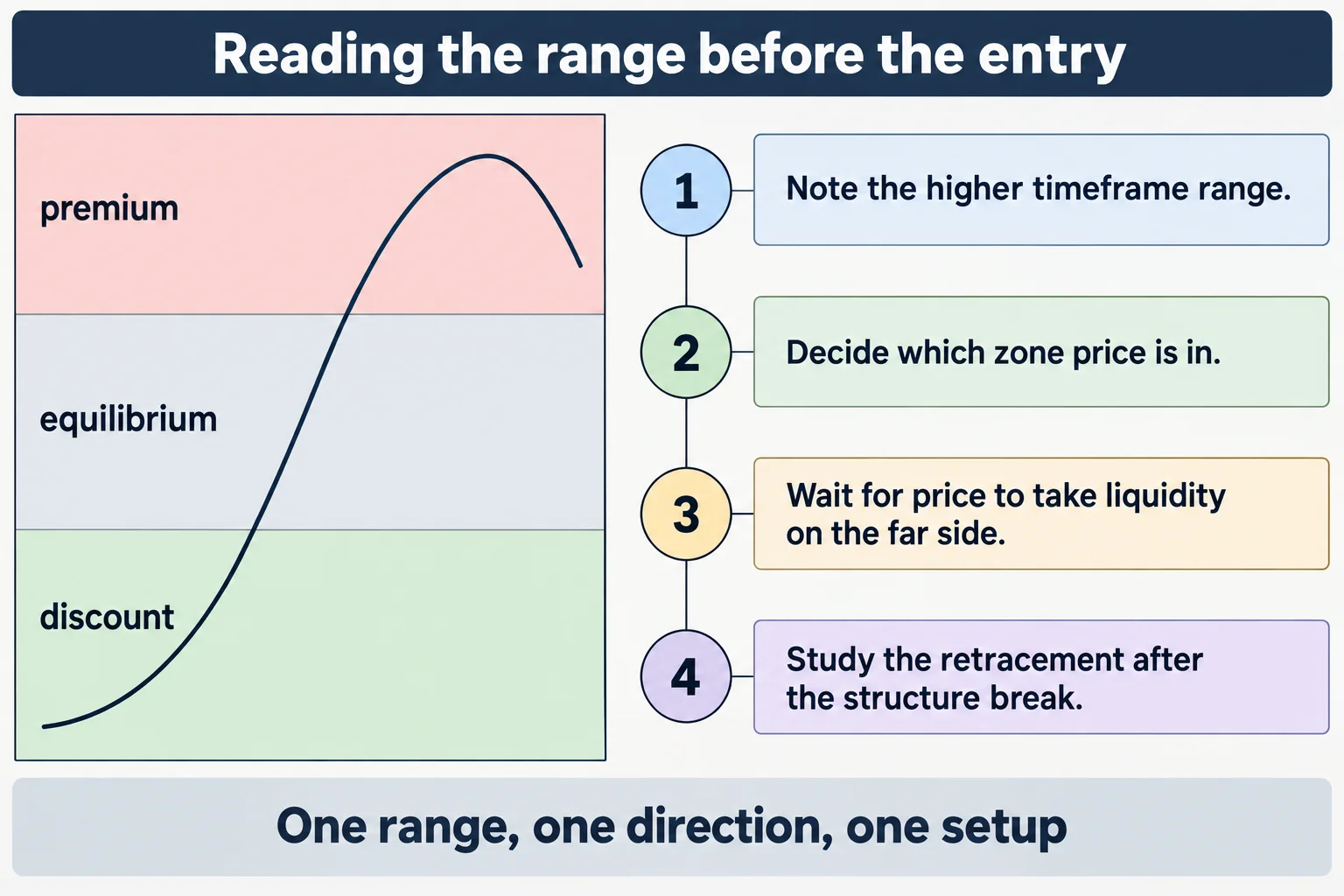
At 9:33 he introduces the premium and discount frame, and at 9:46 says the analysis starts on the daily chart. At 10:30 he restates the question as where price sits in the premium or discount range, and at 10:46 points to a large displacement candle he says caused a buy-side imbalance and sell-side inefficiency that was cleaned up by the drop back. At 10:55 he adds that he does not need that inefficiency to frame the setup.
The range itself is built from a rolling daily lookback. At 17:32 he ties the market structure to the current dealing range, at 17:38 says starting it from the daily chart matters because much bank dealing analysis is formed against daily open, high, low and close, and at 17:53 gives the windows as the last 20, 40 and 60 trading days. At 18:01 he describes the data range as dynamic because it moves forward with the calendar, and at 18:11 reminds viewers not to count Sundays – the same exclusion rule used in the sibling models. The transcript renders the term as the “IP data range” or “if data range” in places; the acronym is not defined in this recording, so it is reported as rendered.
He then argues the whole assembly is not new. At 20:41 he says breakers, order blocks and market structure breaks were already taught in the free tutorials, and that the premium-to-discount matrix relative to the dealing range came in the month-five content. At 20:57 he says that when they are applied together everything dovetails. That is his assessment of his own material’s coherence, and it is worth reading as such.
Time Frames and the 62% Retracement Example
At 21:20 he acknowledges that daily market structure is sometimes unclear and sets the descent: drop to a four-hour chart, and if nothing appears there, down to the one-hour chart, and at 21:38 he states the limit explicitly as nothing lower than that for this purpose. Execution later drops to 15 minutes, so the constraint applies to establishing the premise rather than to the entry chart.
The illustrated entry begins with a retracement measurement. At 14:33 he describes a 62 to 79% retracement band, at 14:35 identifies that band as the optimal trade entry, and at 23:50 lands on the 62% level on the example chart. At 23:57 he says the next step is to wait for a Monday, Tuesday or Wednesday for price to trade down into it, and at 24:05 notes the range was defined using the earlier data ranges. At 24:12 he identifies the last high as the target that keeps the bullish bias active until it is run or taken out.
At 24:24 he drops to the 15-minute chart, at 24:29 notes Sunday’s trading and that Monday did not reach the optimal trade entry, and at 24:38 says Tuesday dropped into it. At 24:51 he identifies the time of day as the New York open and says a buyer could enter there. The targets are prior daily highs: at 25:06 he takes the first objective from the last 20 days as the previous day’s high, and at 25:37 and 25:47 adds the previous Friday’s high and the Wednesday of the previous week’s high. At 26:05 he says the market should target those and that he will stay with it for now.
One number in that passage is worth handling carefully. At 25:09 the transcript reads a high as “60 741”, which is plausible only if the quote convention is understood; a five-digit New Zealand dollar quote would place that level near 0.6074 rather than 6074. The level is therefore left unreproduced here rather than guessed at. The speaker’s method of measuring the retracement with candle bodies rather than wicks, mentioned in the same section, is stated at 24:19 in the accompanying discussion of how he marks the range.
What He Says About Study, Sample Size and Failure
The most useful passage in the lecture is about how a student should judge the model. At 6:54 he says it does not matter what he or anyone else says, and at 6:58 tells viewers not to look outwardly for approval but to find it in the utilization, the sample size and the forward data – explicitly not just backwards data. Read plainly, that is an instruction to test the method on data the model has not already seen, which is the same standard this article applies to the claims that follow it.
He is also direct about losses. At 14:47 he says you simply have to accept a loss, at 14:51 describes the case where the pattern appears and the trade is stopped out, and at 14:56 states that this is not where 100% accuracy is taught – the transcript reads “you don’t learn 100% trading here”. At 25:35 in the example section he also notes he is running through a single pair and that a student should look across a basket, including a cross such as pound-yen or euro-yen.
The Compounding Illustration and What It Is Not
From about 30:30 the recording moves from method to arithmetic. At 30:42 he frames the aim as finding one 25-to-30-pip scalp a week, and at 30:47 builds a compounding illustration on an assumed 2% return per week, which he says compounds to over 100% a year, with an 11,000-dollar figure growing past a million in ten years. At 31:04 he extends the illustration to 6% a month and 1.5% compounded weekly on a self-directed account funded with 1,000 dollars plus 25 dollars a week. At 31:24 he raises taxation on those accounts, and at 31:32 says he will not counsel viewers on which structure to use and that they must research it themselves.
These figures are conditional arithmetic, not results. A 2% weekly return with no losing weeks is the premise of the illustration, not something the recording establishes, and the transcript supplies no win rate, no sample, no transaction costs, no slippage and no drawdown analysis. The same section reaches its most promotional pitch at 33:25, where he says the potential growth and velocity behind compounding small weekly captures is beyond the viewer’s imagination, and at 33:38 he restates the discipline – not day trading every day, but looking for one specific setup. At 33:52 he says this is the model he used when people came to sit with him for a week, and at 34:07 he asks newer traders why they would want to do anything more than learn this well. Whether one setup a week exists at the frequency implied is exactly the kind of question his own instruction at 6:58 says to settle with forward data.
The Lecture as a Study Checklist
- Mark one clearly defined higher-time-frame dealing range, starting on the daily chart and going no lower than the one-hour chart for context (17:38, 21:38).
- Classify the current location as premium, equilibrium or discount relative to that range (9:33, 10:30).
- Wait for a prior high or low to be taken in the expected direction of the setup (15:00, 16:36).
- Require displacement that breaks short-term structure rather than assuming the reversal from the sweep alone (17:05).
- Study the return into the breaker as the entry area, using a 62 to 79% retracement measured with candle bodies (15:42, 14:33).
- Time the entry toward Monday, Tuesday or Wednesday and a session window, with prior daily highs or lows as objectives (23:57, 25:06).
- Judge it on forward data and sample size, not on the educator’s endorsement (6:54).
What the Recording Does Not Establish
The source used here is the video’s own captions, not automatic speech recognition, and no chart was seen. Captions still misplace figures and terms: the data-range acronym appears variously as the “IP data range” and “if data range” at 17:53 and 25:03, the transcript renders “order flow” as “overflow” at 11:34, and the example level at 25:09 cannot be reproduced without knowing the quote convention. None of these were silently corrected.
Several things a reader might want are absent. There is no account statement, no broker confirmation, no sample size, no win rate, no transaction-cost or slippage treatment and no drawdown profile. The 25-to-30-pip weekly scalp and the 2% weekly return are stated aims and assumptions used to build an illustration, not measured outcomes. The example is a single week of a single pair, and the speaker himself says at 25:35 that it is where he would stay for the moment, which is a statement about a working bias rather than a closed result. The claim that the assembled concepts dovetail perfectly at 20:57 is his own assessment of his teaching, and the recording contains nothing independent of his own chart reading that would support or refute it.
Watch the ICT Price Action Model 1 Recording
The recording runs about 43 minutes 45 seconds and is the only primary source used here. The channel is The Inner Circle Trader on YouTube. Because the lecture is delivered over charts, watching it is the only way to see the ranges, breakers and retracement levels described above.
Resources
These are the sources checked for this article. The Federal Reserve series is the official publication of exchange-rate data for the pair used in the example, and the CFTC pages are regulator and investor-education material. None of it is an assessment of ICT, of Price Action Model 1 or of anything said in the recording. Copies, notes and second-hand summaries of this charter lecture circulating elsewhere are unofficial and untested here.
- [1] ICT Charter Price Action Model 1 \ Amplified Lecture – The Inner Circle Trader (primary source; watch page read 15 September 2026, 43M45S)
- [2] Federal Reserve H.10 via FRED – U.S. Dollars to New Zealand Dollar Spot Exchange Rate, daily noon buying rates (the official series for the pair in the example; read 15 September 2026)
- [3] CFTC – Commitments of Traders explanatory notes (background on how commercial and non-commercial trader categories are classified; read 15 September 2026)
- [4] CFTC Learn & Protect – Forex Frauds (the CFTC states that two out of three retail foreign exchange traders lose money each quarter; read 15 September 2026)
This is independent educational commentary on one charter lecture. It is not official ICT material, it is not a tested trading system, and it is not investment advice. The compounding figures discussed in the recording are illustrations built on assumed weekly returns, and the pip and level figures are the speaker’s own statements rather than verified results. Leveraged and foreign exchange trading involves substantial risk and is not suitable for everyone.