
Key takeaways
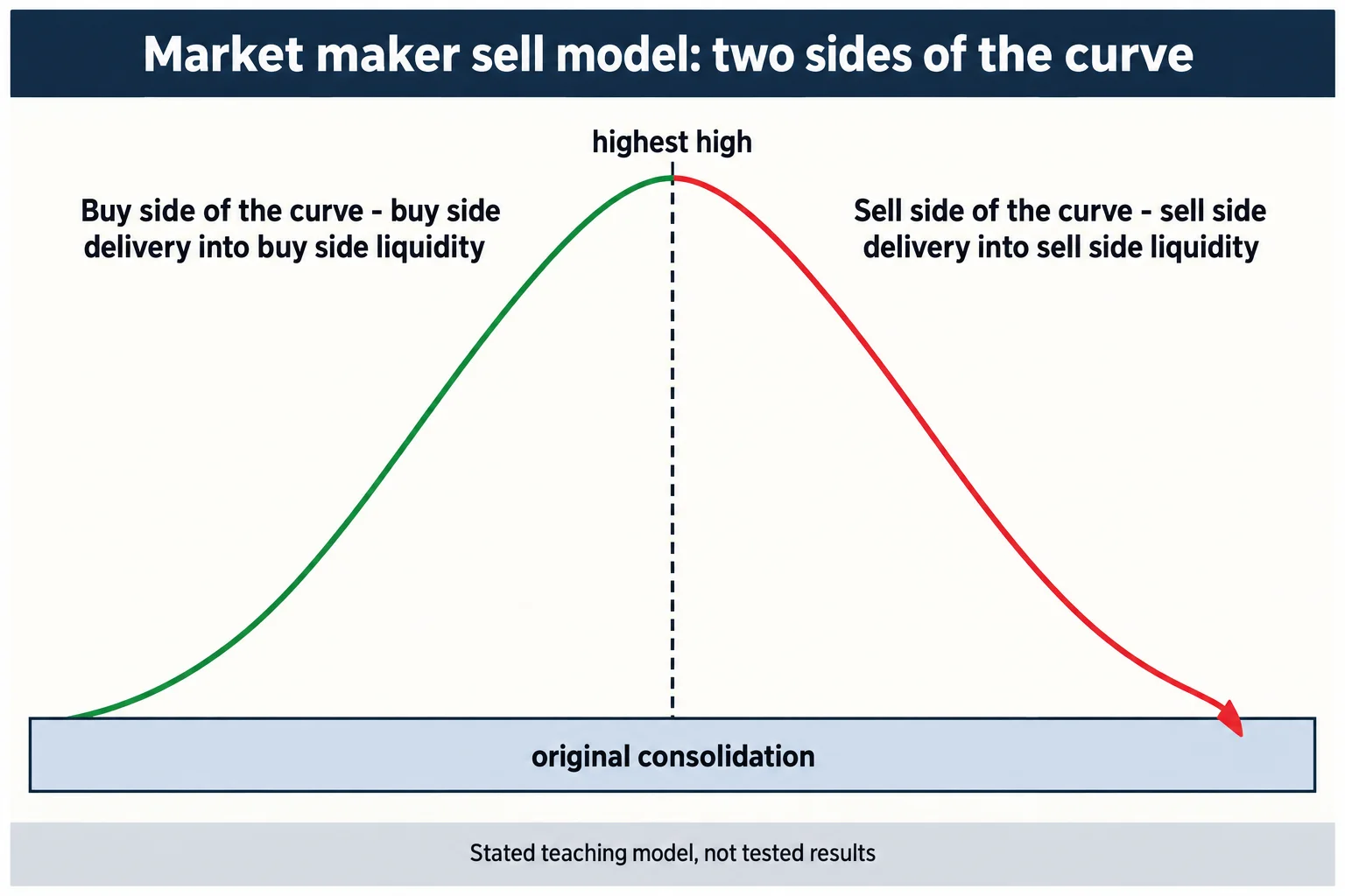
In ICT Mentorship 2023 \ Market Maker Models, ICT presents what he calls a market maker sell model: a swing read as buy side delivery up into resting buy side liquidity, a reversal, then sell side delivery down into sell side liquidity that formed during the rise.
Read the full summary
In ICT Mentorship 2023 \ Market Maker Models, ICT presents what he calls a market maker sell model: a swing read as buy side delivery up into resting buy side liquidity, a reversal, then sell side delivery down into sell side liquidity that formed during the rise. The distinctions he draws are precise and worth keeping separate – delivery is price moving; liquidity is a resting order level (10:30, 11:11). He divides the whole swing at its highest high into a buy side and a sell side of the curve, anchors the structure on what he calls the original consolidation, and later adds a time layer over a GBP/USD example – a return to consolidation at the London open, the upside objective into the New York open, and the downside objective inside the London close window (53:42, 57:00). He states the presentation was done live with no market replay (46:46), and he also says the pattern is hindsight-friendly: many examples only become clear after the move. The recording contains no prices, no fills, no costs and no performance data, and this article does not supply any.
How we researched this article
BestProps used document-based research from primary firm sources, checked September 24, 2026. The complete source list, scope, limitations, and commercial-state record appear near the end of this article.
This is a summary of ICT’s stated framework, not evidence that it works. The captions establish what he said; they cannot verify the chart markings he was reading, and nothing in the recording is presented as a tested result. Where the lesson rests on his own interpretation, the article says so.
The stated prerequisites: every PD array, not one
ICT opens at 0:19 by calling this the last teaching lecture on the channel before a break, and at 0:35 describes it as the closest viewpoint to how he trades. He then sets the entry bar unusually high: at 0:48 he says a market maker model depends on already understanding every PD array, and at 1:16 names breakers, mitigation blocks and inversion fair value gaps as things a viewer must recognise for the model to be visible in real time.
He is explicit that recognition often arrives late. At 6:53 he warns the lesson will frustrate anyone expecting something as elementary as the Silver Bullet or his 2022 model, and at 1:41 his prescribed learning routine is to save, mark up and annotate examples after the fact. That is a study method, not a claim that the setup was tradable in real time.
The scope claim comes at 10:09, where he says the ideas are universal and apply wherever there is a price feed – futures, index futures or forex – with the caveat at 3:32 that everything he shows is a sell model and the buy model is the same thing reversed. He confirms at 53:52 that the whole presentation used one GBP/USD forex pair.
Delivery and liquidity are not the same thing
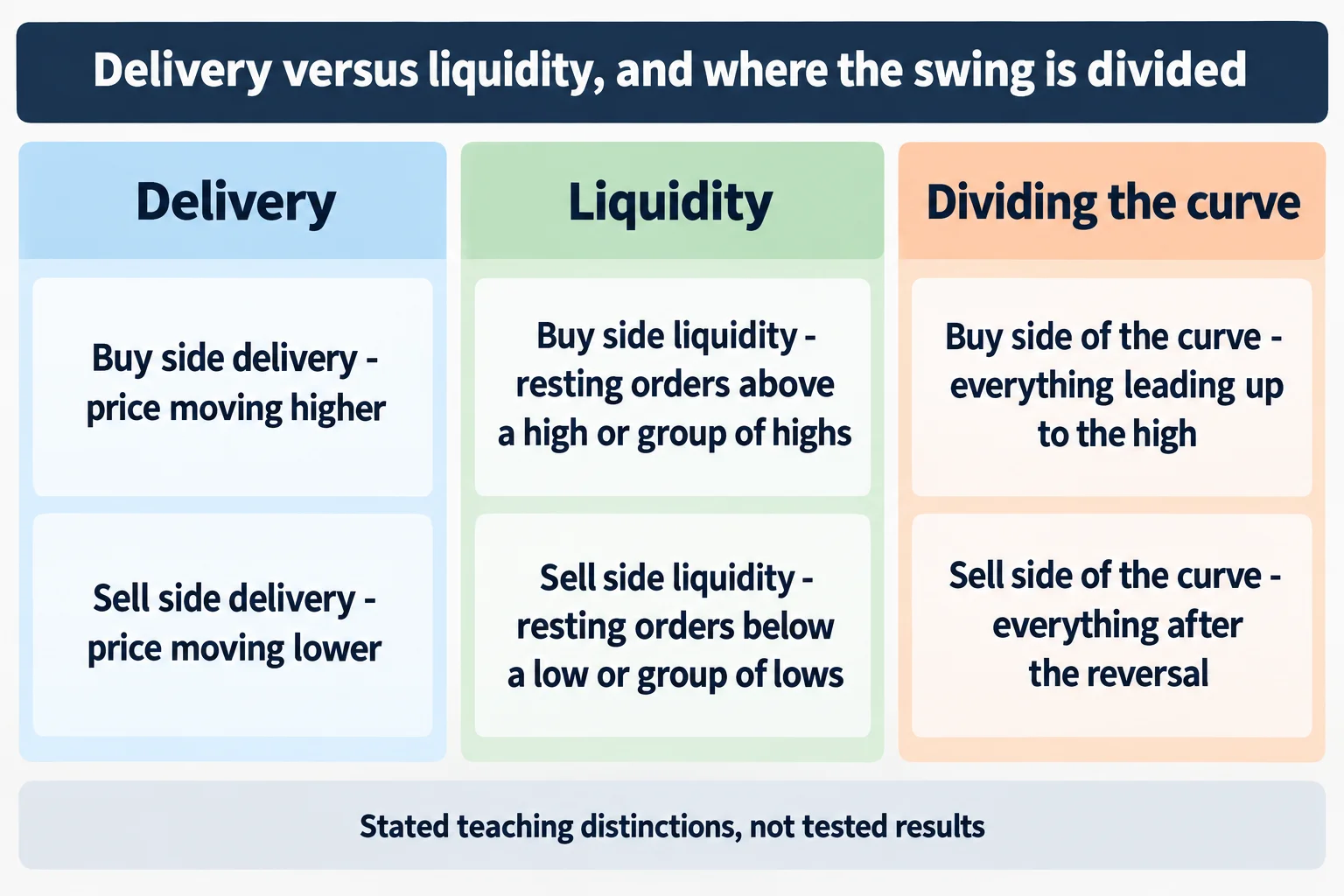
The lesson’s most transferable section is a vocabulary distinction. From 10:30 ICT defines buy side delivery as the actual movement of price higher, and buy side liquidity as the resting orders associated with a single high or a group of highs – breakout buyers or stops protecting shorts (11:11). At 11:24 he sharpens it: liquidity is a stagnant price level or levels where stops reside, while delivery is the animated movement of price toward it. Sell side delivery is the mirror, falling price (11:41).
Applied to the example, the reading becomes: price runs above relative equal highs to engage the liquidity resting there, and once that function is served it can turn and trade back below the low of the prior rally (11:52). At 14:01 he restates that on candlesticks: the rally is buy side delivery, the subsequent drop is sell side delivery attacking the sell side liquidity created by the rally.
He gives two reasons price rises at 14:19 – to reach buy side liquidity, or to revisit an inefficiency. That is where the fair value gap enters as an alternative objective (13:01), and he keeps the two separate rather than treating them as one signal.
The narrative requirement, and why equal highs are not enough
ICT insists the shape alone is not the model. He distinguishes two scenarios that look identical on a chart: a market rising as part of a longer advance, and a market rising to reach a level before a larger decline (17:02). At 49:06 he dismisses the mechanical version of the idea outright, saying that treating a broken high as automatic support does not work, and at 49:09 that what matters is knowing where price is drawn and why.
He also pushes against reading levels as classic support and resistance, saying at 30:30 that he attacks those levels rather than trading them, and listing retail support-and-resistance, harmonic patterns and Elliott wave as things he is targeting (30:51). That is his stated framing of opposing participants, not an established fact about who trades those levels.
Where the lesson does get specific about confirmation, it is about candle bodies. At 16:02 he says wicks piercing a higher-time-frame gap are permissible but the bodies carry the information, and at 47:37 repeats that bodies staying inside the 60-minute array while highs or lows pierce it support his bearish read. That is his chart-reading interpretation, given over charts this article cannot see.
The original consolidation and the two sides of the curve
The structural anchor of the model is what he calls the original consolidation. From 27:09 he explains how he frames it – look for a repetitive or reoccurring level that price keeps referring back to inside the range and use its smooth edge as the consolidation high and the lowest low as the low (27:53). He calls that area accumulation (27:33) and expects price to leave it, reach an objective above, and later offer a return to it (28:06).
The swing is then split at its highest point. At 46:57 he describes an imaginary line at the highest high: everything leading up to it is the buy side of the curve, and everything after the reversal is the sell side of the curve. The sell side objective is the original consolidation low, because that is where sell side liquidity sits – the stops of traders who rode the move up (47:29, 47:36).
He also explains how the same array changes meaning across the divide. At 51:51 he points to a down-close candle that was a bullish order block offering support on the way up, then notes that on the right side of the curve it is read the other way. That is his inversion logic, and it is the part of the model most dependent on the chart he was looking at.
Accumulation, reaccumulation, distribution, redistribution
ICT labels stages, and then explicitly allows the labels to differ between observers. At 37:18 he offers a first-stage accumulation with a second-stage reaccumulation for a viewer who has framed the consolidation correctly, and at 37:46 gives the alternative for someone who has not – a bullish order block as first-stage accumulation instead. At 37:50 he says plainly that the second reading is not wrong.
The sell side gets the same treatment. A bearish breaker becomes first-stage distribution at 48:24, with a fair value gap and breaker combination as the short trigger at 48:36, and a later re-entry on the way down as second-stage redistribution and a pyramiding entry at 53:25. He also gives a concrete management habit there: at 53:35 he says roughly 80% of the position would come off into the original consolidation, and the rest stays only if the market shows it can go deeper.
That flexibility is the honest limit of the framework as a signal. If the same chart supports multiple valid stage labels, the labelling cannot by itself specify a repeatable entry. What it does specify is where the trader is looking and why.
Time frames and the time-of-day layer
The presentation steps from a 60-minute reference area down to 15-minute and five-minute detail. At 27:04 he corrects himself on the time frame mid-explanation – a small slip he catches in the recording – and at 46:35 says he often works on a one-minute chart.
He then layers session times onto the same structure, and this is the most checkable part of the lesson because he names hours. On the GBP/USD example: the return to the original consolidation happens at the London open (54:42), the run into the buy side objective and the reversal land at the New York open, which he calls 7 o’clock in the morning (54:56), and the downside objective falls inside the London close window of 10 o’clock to noon New York local time (57:00). He adds that the breaker, the bearish order block and the trade entry all sit inside the New York open kill zone (55:13).
He reads the sequence as a layered confluence, saying at 54:19 that time sets the stage and price supplies the precision, and he maps the same trade to what he calls the 2022 model at 55:29, then to a Silver Bullet window of 7 to 9 a.m. New York at 55:45. Those are cross-references to his own prior teachings, not independent confirmations, and the fair value gaps he is pointing at are on charts the captions cannot reproduce.
What the lesson does not establish
Several things a reader might expect are absent. The transcript contains no price levels, no pip figures, no position sizes, no transaction costs and no performance data – a text search of the full caption track finds no price or pip values at all. No fill, statement or account record appears anywhere in the recording. He does say at 46:46 that he was executing and annotating live with no market replay, and at 46:30 that he was making the entries as he narrated. That is his account of the session; it is not evidence of profitability, and no result is reported either way.
One term needs flagging rather than quiet correction. The caption track renders the three-candle gap pattern inconsistently – it appears as a close-up-body gap phrase at 15:15 and as an up-close variant later. Both are the automated captions’ rendering of a term he uses without spelling out, so this article describes the pattern structurally instead of adopting either spelling.
Finally, the model’s central input – the directional narrative – has no stated test. Asked how a trader is supposed to know whether a rise is part of a larger advance or a setup for a decline, the recording answers with study and familiarity, and at 49:19 he says that hypothetical lines alone will not get a trader there. That is a real limitation of the framework as presented, and the article states it rather than filling the gap.
Practical takeaways
- Keep delivery and liquidity separate in your notes: movement versus a resting level where stops sit (11:24).
- Frame the original consolidation from a repeated or overlapping level rather than picking an arbitrary range (27:53).
- Divide the swing at its highest high and name what each side is delivering toward (46:57).
- Do not treat a stage label as a signal – the lesson itself allows two valid labellings of one chart (37:50).
- Log session timing alongside the structure, and separate his stated session expectations from anything you have actually tested (57:00).
- Annotate examples after the fact as he instructs, but do not let hindsight recognition stand in for a tested rule (1:41).
Studying this lesson is useful for chart annotation and for learning a consistent vocabulary. It does not provide a rule you can hand to a system, and it makes no claim that these patterns produce profitable results. Leveraged forex and futures trading carries substantial risk.
Watch the original recording
This article draws on the timestamped English captions of the recording, which were generated automatically by YouTube. The recording itself is the primary source and remains the only way to see the chart markings the lesson depends on.
Watch the original recording on YouTube
The video cannot be played inside another website. When its embedded player was loaded and clicked from a BestProps page on 15 September 2026, the player itself reported “Video unavailable — Playback on other websites has been disabled by the video owner.” and stayed on a “Watch on YouTube” prompt with no playback progress at all; the public watch page plays normally. That is why no embed is left here.
Watch ICT Mentorship 2023 \ Market Maker Models on YouTube ↗
The recording runs about 59 minutes and is the only primary source used for this article. The channel is The Inner Circle Trader on YouTube.
Resources
These are the sources checked for this article. The CFTC and Investor.gov pages are general regulator and investor-education material – on leveraged foreign-exchange fraud, on trading systems sold online, and on what leverage is. They are not assessments of ICT or of anything said in the recording. Third-party copies, notes and indicator bundles derived from his material circulate outside his own distribution and were not tested here.
- [1] ICT Mentorship 2023 \ Market Maker Models – The Inner Circle Trader (primary source; watch page read 15 September 2026, 58M37S)
- [2] CFTC Learn & Protect – Forex Frauds (read 15 September 2026)
- [3] CFTC – Fraud Advisory: Commodity Trading Systems Sold on the Internet (read 15 September 2026)
- [4] Investor.gov – Glossary: Leverage (read 15 September 2026)
This is independent educational commentary on one free mentorship lesson. It is not official ICT material, it is not a tested trading system, and it is not investment advice. The speaker describes making entries live during the recording; no fill, account record or performance figure is reported or verified here. Leveraged foreign-exchange and futures trading involves substantial risk and is not suitable for everyone.